pgr_TSPeuclidean - pgRouting Manual (3.3)

pgr_TSPeuclidean
-
pgr_TSPeuclidean- Aproximation using metric algorithm.

Availability:
-
Version 3.2.1
-
Metric Algorithm from Boost library
-
Simulated Annealing Algorithm no longer supported
-
The Simulated Annealing Algorithm related parameters are ignored: max_processing_time, tries_per_temperature, max_changes_per_temperature, max_consecutive_non_changes, initial_temperature, final_temperature, cooling_factor, randomize
-
-
-
Version 3.0.0
-
Name change from pgr_eucledianTSP
-
-
Version 2.3.0
-
New Official function
-
Description
Problem Definition
The travelling salesperson problem (TSP) asks the following question:
Given a list of cities and the distances between each pair of cities, which is the shortest possible route that visits each city exactly once and returns to the origin city?
General Characteristics
-
This problem is an NP-hard optimization problem.
-
Metric Algorithm is used
-
Implementation generates solutions that are twice as long as the optimal tour in the worst case when:
-
Graph is undirected
-
Graph is fully connected
-
Graph where traveling costs on edges obey the triangle inequality.
-
-
On an undirected graph:
-
The traveling costs are symmetric:
-
Traveling costs from
utovare just as much as traveling fromvtou
-
Characteristics
-
Duplicated identifiers with different coordinates are not allowed
-
The coordinates are quite the same for the same identifier, for example
1, 3.5, 1
1, 3.499999999999 0.9999999
-
The coordinates are quite different for the same identifier, for example
2 , 3.5, 1.0
2 , 3.6, 1.1
-
Any duplicated identifier will be ignored. The coordinates that will be kept is arbitrarly.
-
Signatures
Summary
pgr_TSPeuclidean(Coordinates SQL, [start_id], [end_id])
RETURNS SETOF (seq, node, cost, agg_cost)
- Example :
-
With default values
SELECT * FROM pgr_TSPeuclidean(
    $$
    SELECT id, st_X(the_geom) AS x, st_Y(the_geom)AS y  FROM edge_table_vertices_pgr
    $$);
 seq  node       cost         agg_cost
-----+------+----------------+---------------
   1     1               0              0
   2     2               1              1
   3     8   1.41421356237  2.41421356237
   4     7               1  3.41421356237
   5    14   1.58113883008  4.99535239246
   6    15             1.5  6.49535239246
   7    13             0.5  6.99535239246
   8    17             1.5  8.49535239246
   9    12   1.11803398875  9.61338638121
  10     9               1  10.6133863812
  11    16  0.583095189485  11.1964815707
  12     6  0.583095189485  11.7795767602
  13    11               1  12.7795767602
  14    10               1  13.7795767602
  15     5               1  14.7795767602
  16     4    2.2360679775  17.0156447377
  17     3               1  18.0156447377
  18     1   1.41421356237     19.4298583
(18 rows)
Parameters
|
Parameter |
Type |
Default |
Description |
|---|---|---|---|
|
Coordinates SQL |
|
An SQL query, described in the Coordinates SQL section |
|
|
start_vid |
|
|
The first visiting vertex
|
|
end_vid |
|
|
Last visiting vertex before returning to
|
Inner query
Coordinates SQL
Coordinates SQL : an SQL query, which should return a set of rows with the following columns:
|
Column |
Type |
Description |
|---|---|---|
|
id |
|
Identifier of the starting vertex. |
|
x |
|
X value of the coordinate. |
|
y |
|
Y value of the coordinate. |
Result Columns
Returns SET OF
      (seq,


      node,


      cost,


      agg_cost)
|
Column |
Type |
Description |
|---|---|---|
|
seq |
|
Row sequence. |
|
node |
|
Identifier of the node/coordinate/point. |
|
cost |
|
Cost to traverse from the current
|
|
agg_cost |
|
Aggregate cost from the
|
Additional Examples
- Example :
-
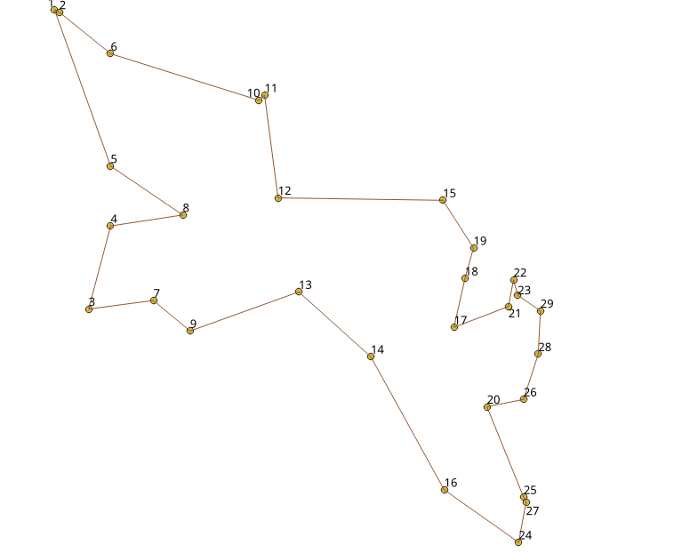
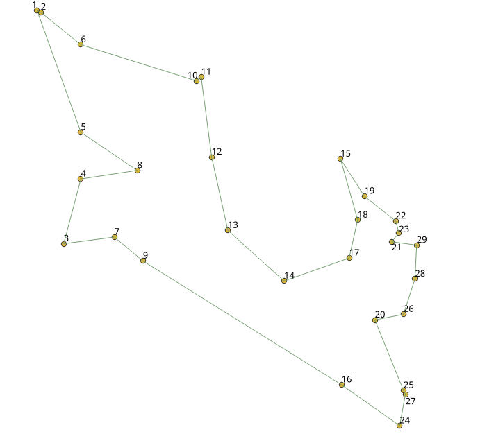
Test 29 cities of Western Sahara
This example shows how to make performance tests using University of Waterloo’s example data using the 29 cities of Western Sahara dataset
Creating a table for the data and storing the data
CREATE TABLE wi29 (id BIGINT, x FLOAT, y FLOAT, geom geometry);
INSERT INTO wi29 (id, x, y) VALUES
(1,20833.3333,17100.0000),
(2,20900.0000,17066.6667),
(3,21300.0000,13016.6667),
(4,21600.0000,14150.0000),
(5,21600.0000,14966.6667),
(6,21600.0000,16500.0000),
(7,22183.3333,13133.3333),
(8,22583.3333,14300.0000),
(9,22683.3333,12716.6667),
(10,23616.6667,15866.6667),
(11,23700.0000,15933.3333),
(12,23883.3333,14533.3333),
(13,24166.6667,13250.0000),
(14,25149.1667,12365.8333),
(15,26133.3333,14500.0000),
(16,26150.0000,10550.0000),
(17,26283.3333,12766.6667),
(18,26433.3333,13433.3333),
(19,26550.0000,13850.0000),
(20,26733.3333,11683.3333),
(21,27026.1111,13051.9444),
(22,27096.1111,13415.8333),
(23,27153.6111,13203.3333),
(24,27166.6667,9833.3333),
(25,27233.3333,10450.0000),
(26,27233.3333,11783.3333),
(27,27266.6667,10383.3333),
(28,27433.3333,12400.0000),
(29,27462.5000,12992.2222);
Adding a geometry (for visual purposes)
UPDATE wi29 SET geom = ST_makePoint(x,y);
Getting a total cost of the tour, compare the value with the length of an optimal tour is 27603, given on the dataset
SELECT *
FROM pgr_TSPeuclidean($$SELECT * FROM wi29$$)
WHERE seq = 30;
 seq  node      cost         agg_cost
-----+------+---------------+---------------
  30     1  2266.91173136  28777.4854127
(1 row)
Getting a geometry of the tour
WITH
tsp_results AS (SELECT seq, geom FROM pgr_TSPeuclidean($$SELECT * FROM wi29$$) JOIN wi29 ON (node = id))
SELECT ST_MakeLine(ARRAY(SELECT geom FROM tsp_results ORDER BY seq));
                                                                                                                                                                                                                                                                                                                                                                                                                                                                                                    st_makeline
--------------------------------------------------------------------------------------------------------------------------------------------------------------------------------------------------------------------------------------------------------------------------------------------------------------------------------------------------------------------------------------------------------------------------------------------------------------------------------------------------------------------------------------------------------------------------------------------------------------------------------------------------------------------------------------------------------------------------------------------------------------------------------------------------------------------------------------------------------------------------------------------------------------------------------------------------------------------------------------------------------------------
 01020000001E000000F085C9545558D4400000000000B3D040000000000069D440107A36ABAAAAD040000000000018D54000000000001DD040107A36AB2A10D7401FF46C5655FDCE40000000000025D740E10B93A9AA1ECF40F085C954D552D740E10B93A9AA62CC40107A36ABAA99D7400000000000E1C940107A36AB4A8FD840E10B93A9EA26C840F085C954D5AAD9401FF46C5655EFC840F085C95455D0D940E10B93A9AA3CCA40F085C9545585D940000000000052CC400000000080EDD94000000000000DCB40A52C431C0776DA40E10B93A9EA33CA40A52C431C6784DA40E10B93A9AAC9C940A52C431C8764DA402C6519E2F87DC94000000000A0D1DA4096B20C711C60C940F085C95455CADA40000000000038C840F085C9545598DA40E10B93A9AA03C740F085C954551BDA40E10B93A9AAD1C640F085C9545598DA40000000000069C440107A36ABAAA0DA40E10B93A9AA47C440107A36ABAA87DA40E10B93A9AA34C340000000008089D94000000000009BC440F085C954D526D6401FF46C5655D6C840F085C954D5A9D540E10B93A9AAA6C9400000000000CDD4401FF46C56556CC940000000000018D5400000000000A3CB40F085C954D50DD6400000000000EECB40000000000018D5401FF46C56553BCD40F085C9545558D4400000000000B3D040
(1 row)
Visualy, The first image is the
optimal solution
and
the second image is the solution obtained with
pgr_TSPeuclidean
.
See Also
-
Sample Data network.
-
Metric Algorithm from Boost library
Indices and tables