Chapter 4. Using PostGIS: Data Management and Queries
- 4.1. GIS Objects
- 4.2. PostGIS Geography Type
- 4.3. Using OpenGIS Standards
-
- 4.3.1. The SPATIAL_REF_SYS Table and Spatial Reference Systems
- 4.3.2. The GEOMETRY_COLUMNS VIEW
- 4.3.3. Creating a Spatial Table
- 4.3.4. Manually Registering Geometry Columns in geometry_columns
- 4.3.5. Ensuring OpenGIS compliancy of geometries
- 4.3.6. Dimensionally Extended 9 Intersection Model (DE-9IM)
- 4.4. Loading GIS (Vector) Data
- 4.5. Retrieving GIS Data
- 4.6. Building Indexes
- 4.7. Complex Queries
The GIS objects supported by PostGIS are a superset of the "Simple Features" defined by the OpenGIS Consortium (OGC). PostGIS supports all the objects and functions specified in the OGC "Simple Features for SQL" specification.
PostGIS extends the standard with support for 3DZ, 3DM and 4D coordinates.
The OpenGIS specification defines two standard ways of expressing spatial objects: the Well-Known Text (WKT) form and the Well-Known Binary (WKB) form. Both WKT and WKB include information about the type of the object and the coordinates which form the object.
Examples of the text representations (WKT) of the spatial objects of the features are as follows:
-
POINT(0 0)
-
LINESTRING(0 0,1 1,1 2)
-
POLYGON((0 0,4 0,4 4,0 4,0 0),(1 1, 2 1, 2 2, 1 2,1 1))
-
MULTIPOINT((0 0),(1 2))
-
MULTILINESTRING((0 0,1 1,1 2),(2 3,3 2,5 4))
-
MULTIPOLYGON(((0 0,4 0,4 4,0 4,0 0),(1 1,2 1,2 2,1 2,1 1)), ((-1 -1,-1 -2,-2 -2,-2 -1,-1 -1)))
-
GEOMETRYCOLLECTION(POINT(2 3),LINESTRING(2 3,3 4))
The OpenGIS specification also requires that the internal storage format of spatial objects include a spatial referencing system identifier (SRID). The SRID is required when creating spatial objects for insertion into the database.
Input/Output of these formats are available using the following interfaces:
bytea WKB = ST_AsBinary(geometry);
text WKT = ST_AsText(geometry);
geometry = ST_GeomFromWKB(bytea WKB, SRID);
geometry = ST_GeometryFromText(text WKT, SRID);
For example, a valid insert statement to create and insert an OGC spatial object would be:
INSERT INTO geotable ( the_geom, the_name )
  VALUES ( ST_GeomFromText('POINT(-126.4 45.32)', 312), 'A Place');
OGC formats only support 2D geometries, and the associated SRID is *never* embedded in the input/output representations.
PostGIS extended formats are currently superset of OGC one (every valid WKB/WKT is a valid EWKB/EWKT) but this might vary in the future, specifically if OGC comes out with a new format conflicting with our extensions. Thus you SHOULD NOT rely on this feature!
PostGIS EWKB/EWKT add 3DM, 3DZ, 4D coordinates support and embedded SRID information.
Examples of the text representations (EWKT) of the extended spatial objects of the features are as follows.
-
POINT(0 0 0) -- XYZ
-
SRID=32632;POINT(0 0) -- XY with SRID
-
POINTM(0 0 0) -- XYM
-
POINT(0 0 0 0) -- XYZM
-
SRID=4326;MULTIPOINTM(0 0 0,1 2 1) -- XYM with SRID
-
MULTILINESTRING((0 0 0,1 1 0,1 2 1),(2 3 1,3 2 1,5 4 1))
-
POLYGON((0 0 0,4 0 0,4 4 0,0 4 0,0 0 0),(1 1 0,2 1 0,2 2 0,1 2 0,1 1 0))
-
MULTIPOLYGON(((0 0 0,4 0 0,4 4 0,0 4 0,0 0 0),(1 1 0,2 1 0,2 2 0,1 2 0,1 1 0)),((-1 -1 0,-1 -2 0,-2 -2 0,-2 -1 0,-1 -1 0)))
-
GEOMETRYCOLLECTIONM( POINTM(2 3 9), LINESTRINGM(2 3 4, 3 4 5) )
-
MULTICURVE( (0 0, 5 5), CIRCULARSTRING(4 0, 4 4, 8 4) )
-
POLYHEDRALSURFACE( ((0 0 0, 0 0 1, 0 1 1, 0 1 0, 0 0 0)), ((0 0 0, 0 1 0, 1 1 0, 1 0 0, 0 0 0)), ((0 0 0, 1 0 0, 1 0 1, 0 0 1, 0 0 0)), ((1 1 0, 1 1 1, 1 0 1, 1 0 0, 1 1 0)), ((0 1 0, 0 1 1, 1 1 1, 1 1 0, 0 1 0)), ((0 0 1, 1 0 1, 1 1 1, 0 1 1, 0 0 1)) )
-
TRIANGLE ((0 0, 0 9, 9 0, 0 0))
-
TIN( ((0 0 0, 0 0 1, 0 1 0, 0 0 0)), ((0 0 0, 0 1 0, 1 1 0, 0 0 0)) )
Conversion between these formats is available using the following interfaces:
bytea EWKB = ST_AsEWKB(geometry);
text EWKT = ST_AsEWKT(geometry);
geometry = ST_GeomFromEWKB(bytea EWKB);
geometry = ST_GeomFromEWKT(text EWKT);
For example, a valid insert statement to create and insert a PostGIS spatial object would be:
INSERT INTO geotable ( the_geom, the_name )
  VALUES ( ST_GeomFromEWKT('SRID=312;POINTM(-126.4 45.32 15)'), 'A Place' )
The "canonical forms" of a PostgreSQL type are the representations you get with a simple query (without any function call) and the one which is guaranteed to be accepted with a simple insert, update or copy. For the PostGIS 'geometry' type these are:
- Output
  - binary: EWKB
	ascii: HEXEWKB (EWKB in hex form)
- Input
  - binary: EWKB
	ascii: HEXEWKB|EWKT
For example this statement reads EWKT and returns HEXEWKB in the process of canonical ascii input/output:
=# SELECT 'SRID=4;POINT(0 0)'::geometry;

geometry
----------------------------------------------------
01010000200400000000000000000000000000000000000000
(1 row)
The SQL Multimedia Applications Spatial specification extends the simple features for SQL spec by defining a number of circularly interpolated curves.
The SQL-MM definitions include 3DM, 3DZ and 4D coordinates, but do not allow the embedding of SRID information.
The Well-Known Text extensions are not yet fully supported. Examples of some simple curved geometries are shown below:
-
CIRCULARSTRING(0 0, 1 1, 1 0)
CIRCULARSTRING(0 0, 4 0, 4 4, 0 4, 0 0)
The CIRCULARSTRING is the basic curve type, similar to a LINESTRING in the linear world. A single segment required three points, the start and end points (first and third) and any other point on the arc. The exception to this is for a closed circle, where the start and end points are the same. In this case the second point MUST be the center of the arc, ie the opposite side of the circle. To chain arcs together, the last point of the previous arc becomes the first point of the next arc, just like in LINESTRING. This means that a valid circular string must have an odd number of points greater than 1.
-
COMPOUNDCURVE(CIRCULARSTRING(0 0, 1 1, 1 0),(1 0, 0 1))
A compound curve is a single, continuous curve that has both curved (circular) segments and linear segments. That means that in addition to having well-formed components, the end point of every component (except the last) must be coincident with the start point of the following component.
-
CURVEPOLYGON(CIRCULARSTRING(0 0, 4 0, 4 4, 0 4, 0 0),(1 1, 3 3, 3 1, 1 1))
Example compound curve in a curve polygon: CURVEPOLYGON(COMPOUNDCURVE(CIRCULARSTRING(0 0,2 0, 2 1, 2 3, 4 3),(4 3, 4 5, 1 4, 0 0)), CIRCULARSTRING(1.7 1, 1.4 0.4, 1.6 0.4, 1.6 0.5, 1.7 1) )
A CURVEPOLYGON is just like a polygon, with an outer ring and zero or more inner rings. The difference is that a ring can take the form of a circular string, linear string or compound string.
As of PostGIS 1.4 PostGIS supports compound curves in a curve polygon.
-
MULTICURVE((0 0, 5 5),CIRCULARSTRING(4 0, 4 4, 8 4))
The MULTICURVE is a collection of curves, which can include linear strings, circular strings or compound strings.
-
MULTISURFACE(CURVEPOLYGON(CIRCULARSTRING(0 0, 4 0, 4 4, 0 4, 0 0),(1 1, 3 3, 3 1, 1 1)),((10 10, 14 12, 11 10, 10 10),(11 11, 11.5 11, 11 11.5, 11 11)))
This is a collection of surfaces, which can be (linear) polygons or curve polygons.
![[Note]](images/note.png)
|
|
|
All floating point comparisons within the SQL-MM implementation are performed to a specified tolerance, currently 1E-8. |
The geography type provides native support for spatial features represented on "geographic" coordinates (sometimes called "geodetic" coordinates, or "lat/lon", or "lon/lat"). Geographic coordinates are spherical coordinates expressed in angular units (degrees).
The basis for the PostGIS geometry type is a plane. The shortest path between two points on the plane is a straight line. That means calculations on geometries (areas, distances, lengths, intersections, etc) can be calculated using cartesian mathematics and straight line vectors.
The basis for the PostGIS geographic type is a sphere. The shortest path between two points on the sphere is a great circle arc. That means that calculations on geographies (areas, distances, lengths, intersections, etc) must be calculated on the sphere, using more complicated mathematics. For more accurate measurements, the calculations must take the actual spheroidal shape of the world into account.
Because the underlying mathematics is much more complicated, there are fewer functions defined for the geography type than for the geometry type. Over time, as new algorithms are added, the capabilities of the geography type will expand.
It uses a data type called
geography
. None of the GEOS functions support the
geography
type. As a workaround one can convert back and forth between geometry and geography types.
Prior to PostGIS 2.2, the geography type only supported WGS 84 long lat (SRID:4326).
For PostGIS 2.2 and above, any long/lat based spatial reference system defined in the
spatial_ref_sys
table can be used.
You can even add your own custom spheroidal spatial reference system as described in
geography type is not limited to earth
.
Regardless which spatial reference system you use, the units returned by the measurement ( ST_Distance , ST_Length , ST_Perimeter , ST_Area ) and for input of ST_DWithin are in meters.
The geography type uses the PostgreSQL typmod definition format so that a table with a geography field can be added in a single step. All the standard OGC formats except for curves are supported.
The geography type does not support curves, TINS, or POLYHEDRALSURFACEs, but other geometry types are supported. Standard geometry type data will autocast to geography if it is of SRID 4326. You can also use the EWKT and EWKB conventions to insert data.
-
POINT: Creating a table with 2D point geography when srid is not specified defaults to 4326 WGS 84 long lat:
CREATE TABLE ptgeogwgs(gid serial PRIMARY KEY, geog geography(POINT) );
POINT: Creating a table with 2D point geography in NAD83 longlat:
CREATE TABLE ptgeognad83(gid serial PRIMARY KEY, geog geography(POINT,4269) );
Creating a table with z coordinate point and explicitly specifying srid
CREATE TABLE ptzgeogwgs84(gid serial PRIMARY KEY, geog geography(POINTZ,4326) );
-
LINESTRING
CREATE TABLE lgeog(gid serial PRIMARY KEY, geog geography(LINESTRING) );
-
POLYGON
--polygon NAD 1927 long lat
CREATE TABLE lgeognad27(gid serial PRIMARY KEY, geog geography(POLYGON,4267) );
-
MULTIPOINT
-
MULTILINESTRING
-
MULTIPOLYGON
-
GEOMETRYCOLLECTION
The geography fields get registered in the
geography_columns
system view.
Now, check the "geography_columns" view and see that your table is listed.
You can create a new table with a GEOGRAPHY column using the CREATE TABLE syntax.
CREATE TABLE global_points (
    id SERIAL PRIMARY KEY,
    name VARCHAR(64),
    location GEOGRAPHY(POINT,4326)
  );
Note that the location column has type GEOGRAPHY and that geography type supports two optional modifiers: a type modifier that restricts the kind of shapes and dimensions allowed in the column; an SRID modifier that restricts the coordinate reference identifier to a particular number.
Allowable values for the type modifier are: POINT, LINESTRING, POLYGON, MULTIPOINT, MULTILINESTRING, MULTIPOLYGON. The modifier also supports dimensionality restrictions through suffixes: Z, M and ZM. So, for example a modifier of 'LINESTRINGM' would only allow line strings with three dimensions in, and would treat the third dimension as a measure. Similarly, 'POINTZM' would expect four dimensional data.
If you do not specify an SRID, the SRID will default to 4326 WGS 84 long/lat will be used, and all calculations will proceed using WGS84.
Once you have created your table, you can see it in the GEOGRAPHY_COLUMNS table:
-- See the contents of the metadata view
SELECT * FROM geography_columns;
You can insert data into the table the same as you would if it was using a GEOMETRY column:
-- Add some data into the test table
INSERT INTO global_points (name, location) VALUES ('Town', 'SRID=4326;POINT(-110 30)');
INSERT INTO global_points (name, location) VALUES ('Forest', 'SRID=4326;POINT(-109 29)');
INSERT INTO global_points (name, location) VALUES ('London', 'SRID=4326;POINT(0 49)');
Creating an index works the same as GEOMETRY. PostGIS will note that the column type is GEOGRAPHY and create an appropriate sphere-based index instead of the usual planar index used for GEOMETRY.
-- Index the test table with a spherical index
  CREATE INDEX global_points_gix ON global_points USING GIST ( location );
Query and measurement functions use units of meters. So distance parameters should be expressed in meters, and return values should be expected in meters (or square meters for areas).
-- Show a distance query and note, London is outside the 1000km tolerance
  SELECT name FROM global_points WHERE ST_DWithin(location, 'SRID=4326;POINT(-110 29)'::geography, 1000000);
You can see the power of GEOGRAPHY in action by calculating how close a plane flying from Seattle to London (LINESTRING(-122.33 47.606, 0.0 51.5)) comes to Reykjavik (POINT(-21.96 64.15)).
-- Distance calculation using GEOGRAPHY (122.2km)
  SELECT ST_Distance('LINESTRING(-122.33 47.606, 0.0 51.5)'::geography, 'POINT(-21.96 64.15)'::geography);
-- Distance calculation using GEOMETRY (13.3 "degrees")
  SELECT ST_Distance('LINESTRING(-122.33 47.606, 0.0 51.5)'::geometry, 'POINT(-21.96 64.15)'::geometry);
Testing different lon/lat projects.
Any long lat spatial reference system listed in
spatial_ref_sys
table is allowed.
-- NAD 83 lon/lat
SELECT 'SRID=4269;POINT(-123 34)'::geography;
                    geography
----------------------------------------------------
 0101000020AD1000000000000000C05EC00000000000004140
(1 row)
-- NAD27 lon/lat
SELECT 'SRID=4267;POINT(-123 34)'::geography;

                    geography
----------------------------------------------------
 0101000020AB1000000000000000C05EC00000000000004140
(1 row)
-- NAD83 UTM zone meters, yields error since its a meter based projection
SELECT 'SRID=26910;POINT(-123 34)'::geography;

ERROR:  Only lon/lat coordinate systems are supported in geography.
LINE 1: SELECT 'SRID=26910;POINT(-123 34)'::geography;
The GEOGRAPHY type calculates the true shortest distance over the sphere between Reykjavik and the great circle flight path between Seattle and London.
Great Circle mapper The GEOMETRY type calculates a meaningless cartesian distance between Reykjavik and the straight line path from Seattle to London plotted on a flat map of the world. The nominal units of the result might be called "degrees", but the result doesn't correspond to any true angular difference between the points, so even calling them "degrees" is inaccurate.
The geography type allows you to store data in longitude/latitude coordinates, but at a cost: there are fewer functions defined on GEOGRAPHY than there are on GEOMETRY; those functions that are defined take more CPU time to execute.
The type you choose should be conditioned on the expected working area of the application you are building. Will your data span the globe or a large continental area, or is it local to a state, county or municipality?
-
If your data is contained in a small area, you might find that choosing an appropriate projection and using GEOMETRY is the best solution, in terms of performance and functionality available.
-
If your data is global or covers a continental region, you may find that GEOGRAPHY allows you to build a system without having to worry about projection details. You store your data in longitude/latitude, and use the functions that have been defined on GEOGRAPHY.
-
If you don't understand projections, and you don't want to learn about them, and you're prepared to accept the limitations in functionality available in GEOGRAPHY, then it might be easier for you to use GEOGRAPHY than GEOMETRY. Simply load your data up as longitude/latitude and go from there.
Refer to Section 14.11, “PostGIS Function Support Matrix” for compare between what is supported for Geography vs. Geometry. For a brief listing and description of Geography functions, refer to Section 14.4, “PostGIS Geography Support Functions”
- 4.2.3.1. Do you calculate on the sphere or the spheroid?
- 4.2.3.2. What about the date-line and the poles?
- 4.2.3.3. What is the longest arc you can process?
- 4.2.3.4. Why is it so slow to calculate the area of Europe / Russia / insert big geographic region here ?
|
4.2.3.1. |
Do you calculate on the sphere or the spheroid? |
|
By default, all distance and area calculations are done on the spheroid. You should find that the results of calculations in local areas match up will with local planar results in good local projections. Over larger areas, the spheroidal calculations will be more accurate than any calculation done on a projected plane. All the geography functions have the option of using a sphere calculation, by setting a final boolean parameter to 'FALSE'. This will somewhat speed up calculations, particularly for cases where the geometries are very simple. |
|
|
4.2.3.2. |
What about the date-line and the poles? |
|
All the calculations have no conception of date-line or poles, the coordinates are spherical (longitude/latitude) so a shape that crosses the dateline is, from a calculation point of view, no different from any other shape. |
|
|
4.2.3.3. |
What is the longest arc you can process? |
|
We use great circle arcs as the "interpolation line" between two points. That means any two points are actually joined up two ways, depending on which direction you travel along the great circle. All our code assumes that the points are joined by the *shorter* of the two paths along the great circle. As a consequence, shapes that have arcs of more than 180 degrees will not be correctly modelled. |
|
|
4.2.3.4. |
Why is it so slow to calculate the area of Europe / Russia / insert big geographic region here ? |
|
Because the polygon is so darned huge! Big areas are bad for two reasons: their bounds are huge, so the index tends to pull the feature no matter what query you run; the number of vertices is huge, and tests (distance, containment) have to traverse the vertex list at least once and sometimes N times (with N being the number of vertices in the other candidate feature). As with GEOMETRY, we recommend that when you have very large polygons, but are doing queries in small areas, you "denormalize" your geometric data into smaller chunks so that the index can effectively subquery parts of the object and so queries don't have to pull out the whole object every time. Please consult ST_Subdivide function documentation. Just because you *can* store all of Europe in one polygon doesn't mean you *should*. |
- 4.3.1. The SPATIAL_REF_SYS Table and Spatial Reference Systems
- 4.3.2. The GEOMETRY_COLUMNS VIEW
- 4.3.3. Creating a Spatial Table
- 4.3.4. Manually Registering Geometry Columns in geometry_columns
- 4.3.5. Ensuring OpenGIS compliancy of geometries
- 4.3.6. Dimensionally Extended 9 Intersection Model (DE-9IM)
The OpenGIS "Simple Features Specification for SQL" defines standard GIS object types, the functions required to manipulate them, and a set of meta-data tables. In order to ensure that meta-data remain consistent, operations such as creating and removing a spatial column are carried out through special procedures defined by OpenGIS.
There are two OpenGIS meta-data tables:
SPATIAL_REF_SYS
and
GEOMETRY_COLUMNS
. The
SPATIAL_REF_SYS
table holds the numeric IDs and textual
descriptions of coordinate systems used in the spatial database.
The spatial_ref_sys table is a PostGIS included and OGC compliant database table that lists over 3000 known spatial reference systems and details needed to transform/reproject between them.
Although the PostGIS spatial_ref_sys table contains over 3000 of the more commonly used spatial reference system definitions that can be handled by the proj library, it does not contain all known to man and you can define your own custom projection if you are familiar with proj4 constructs. Keep in mind that most spatial reference systems are regional and have no meaning when used outside of the bounds they were intended for.
An excellent resource for finding spatial reference systems not defined in the core set is http://spatialreference.org/
Some of the more commonly used spatial reference systems are: 4326 - WGS 84 Long Lat , 4269 - NAD 83 Long Lat , 3395 - WGS 84 World Mercator , 2163 - US National Atlas Equal Area , Spatial reference systems for each NAD 83, WGS 84 UTM zone - UTM zones are one of the most ideal for measurement, but only cover 6-degree regions.
Various US state plane spatial reference systems (meter or feet based) - usually one or 2 exists per US state. Most of the meter ones are in the core set, but many of the feet based ones or ESRI created ones you will need to pull from spatialreference.org .
For details on determining which UTM zone to use for your area of interest, check out the utmzone PostGIS plpgsql helper function .
The
SPATIAL_REF_SYS
table definition is as
follows:
CREATE TABLE spatial_ref_sys (
  srid       INTEGER NOT NULL PRIMARY KEY,
  auth_name  VARCHAR(256),
  auth_srid  INTEGER,
  srtext     VARCHAR(2048),
  proj4text  VARCHAR(2048)
)
The
SPATIAL_REF_SYS
columns are as
follows:
- SRID
-
An integer value that uniquely identifies the Spatial Referencing System (SRS) within the database.
- AUTH_NAME
-
The name of the standard or standards body that is being cited for this reference system. For example, "EPSG" would be a valid
AUTH_NAME. - AUTH_SRID
-
The ID of the Spatial Reference System as defined by the Authority cited in the
AUTH_NAME. In the case of EPSG, this is where the EPSG projection code would go. - SRTEXT
-
The Well-Known Text representation of the Spatial Reference System. An example of a WKT SRS representation is:
PROJCS["NAD83 / UTM Zone 10N",
  GEOGCS["NAD83",
	DATUM["North_American_Datum_1983",
	  SPHEROID["GRS 1980",6378137,298.257222101]
	],
	PRIMEM["Greenwich",0],
	UNIT["degree",0.0174532925199433]
  ],
  PROJECTION["Transverse_Mercator"],
  PARAMETER["latitude_of_origin",0],
  PARAMETER["central_meridian",-123],
  PARAMETER["scale_factor",0.9996],
  PARAMETER["false_easting",500000],
  PARAMETER["false_northing",0],
  UNIT["metre",1]
]
For a listing of EPSG projection codes and their corresponding WKT representations, see http://www.opengeospatial.org/ . For a discussion of WKT in general, see the OpenGIS "Coordinate Transformation Services Implementation Specification" at http://www.opengeospatial.org/standards . For information on the European Petroleum Survey Group (EPSG) and their database of spatial reference systems, see http://www.epsg.org .
- PROJ4TEXT
-
PostGIS uses the Proj4 library to provide coordinate transformation capabilities. The
PROJ4TEXTcolumn contains the Proj4 coordinate definition string for a particular SRID. For example:+proj=utm +zone=10 +ellps=clrk66 +datum=NAD27 +units=m
For more information about, see the Proj4 web site at http://trac.osgeo.org/proj/ . The
spatial_ref_sys.sqlfile contains bothSRTEXTandPROJ4TEXTdefinitions for all EPSG projections.
GEOMETRY_COLUMNS
is a view reading from database system catalogs.
Its structure is as follows:
\d geometry_columns
             View "public.geometry_columns"
      Column       |          Type          | Modifiers
-------------------+------------------------+-----------
 f_table_catalog   | character varying(256) |
 f_table_schema    | character varying(256) |
 f_table_name      | character varying(256) |
 f_geometry_column | character varying(256) |
 coord_dimension   | integer                |
 srid              | integer                |
 type              | character varying(30)  |
The column meanings are:
- F_TABLE_CATALOG, F_TABLE_SCHEMA, F_TABLE_NAME
-
The fully qualified name of the feature table containing the geometry column. Note that the terms "catalog" and "schema" are Oracle-ish. There is not PostgreSQL analogue of "catalog" so that column is left blank -- for "schema" the PostgreSQL schema name is used (
publicis the default). - F_GEOMETRY_COLUMN
-
The name of the geometry column in the feature table.
- COORD_DIMENSION
-
The spatial dimension (2, 3 or 4 dimensional) of the column.
- SRID
-
The ID of the spatial reference system used for the coordinate geometry in this table. It is a foreign key reference to the
SPATIAL_REF_SYS. - TYPE
-
The type of the spatial object. To restrict the spatial column to a single type, use one of: POINT, LINESTRING, POLYGON, MULTIPOINT, MULTILINESTRING, MULTIPOLYGON, GEOMETRYCOLLECTION or corresponding XYM versions POINTM, LINESTRINGM, POLYGONM, MULTIPOINTM, MULTILINESTRINGM, MULTIPOLYGONM, GEOMETRYCOLLECTIONM. For heterogeneous (mixed-type) collections, you can use "GEOMETRY" as the type.
This attribute is (probably) not part of the OpenGIS specification, but is required for ensuring type homogeneity.
Creating a table with spatial data, can be done in one step. As shown in the following example which creates a roads table with a 2D linestring geometry column in WGS84 long lat
CREATE TABLE ROADS (ID serial, ROAD_NAME text, geom geometry(LINESTRING,4326) );
We can add additional columns using standard ALTER TABLE command as we do in this next example where we add a 3-D linestring.
ALTER TABLE roads ADD COLUMN geom2 geometry(LINESTRINGZ,4326);
Two of the cases where you may need this are the case of SQL Views and bulk inserts. For bulk insert case, you can correct the registration in the geometry_columns table by constraining the column or doing an alter table. For views, you could expose using a CAST operation. Note, if your column is typmod based, the creation process would register it correctly, so no need to do anything. Also views that have no spatial function applied to the geometry will register the same as the underlying table geometry column.
-- Lets say you have a view created like this
CREATE VIEW public.vwmytablemercator AS
	SELECT gid, ST_Transform(geom, 3395) As geom, f_name
	FROM public.mytable;

-- For it to register correctly
-- You need to cast the geometry
--
DROP VIEW public.vwmytablemercator;
CREATE VIEW  public.vwmytablemercator AS
	SELECT gid, ST_Transform(geom, 3395)::geometry(Geometry, 3395) As geom, f_name
	FROM public.mytable;

-- If you know the geometry type for sure is a 2D POLYGON then you could do
DROP VIEW public.vwmytablemercator;
CREATE VIEW  public.vwmytablemercator AS
	SELECT gid, ST_Transform(geom,3395)::geometry(Polygon, 3395) As geom, f_name
	FROM public.mytable;
--Lets say you created a derivative table by doing a bulk insert
SELECT poi.gid, poi.geom, citybounds.city_name
INTO myschema.my_special_pois
FROM poi INNER JOIN citybounds ON ST_Intersects(citybounds.geom, poi.geom);

-- Create 2D index on new table
CREATE INDEX idx_myschema_myspecialpois_geom_gist
  ON myschema.my_special_pois USING gist(geom);

-- If your points are 3D points or 3M points,
-- then you might want to create an nd index instead of a 2D index
CREATE INDEX my_special_pois_geom_gist_nd
	ON my_special_pois USING gist(geom gist_geometry_ops_nd);

-- To manually register this new table's geometry column in geometry_columns.
-- Note it will also change the underlying structure of the table to
-- to make the column typmod based.
SELECT populate_geometry_columns('myschema.my_special_pois'::regclass);

-- If you are using PostGIS 2.0 and for whatever reason, you
-- you need the constraint based definition behavior
-- (such as case of inherited tables where all children do not have the same type and srid)
-- set optional use_typmod argument to false
SELECT populate_geometry_columns('myschema.my_special_pois'::regclass, false);
Although the old-constraint based method is still supported, a constraint-based geometry column used directly in a view, will not register correctly in geometry_columns, as will a typmod one. In this example we define a column using typmod and another using constraints.
CREATE TABLE pois_ny(gid SERIAL PRIMARY KEY, poi_name text, cat text, geom geometry(POINT,4326));
SELECT AddGeometryColumn('pois_ny', 'geom_2160', 2160, 'POINT', 2, false);
If we run in psql
\d pois_ny;
We observe they are defined differently -- one is typmod, one is constraint
                                  Table "public.pois_ny"
  Column   |         Type          |                       Modifiers

-----------+-----------------------+------------------------------------------------------
 gid       | integer               | not null default nextval('pois_ny_gid_seq'::regclass)
 poi_name  | text                  |
 cat       | character varying(20) |
 geom      | geometry(Point,4326)  |
 geom_2160 | geometry              |
Indexes:
    "pois_ny_pkey" PRIMARY KEY, btree (gid)
Check constraints:
    "enforce_dims_geom_2160" CHECK (st_ndims(geom_2160) = 2)
    "enforce_geotype_geom_2160" CHECK (geometrytype(geom_2160) = 'POINT'::text
        OR geom_2160 IS NULL)
    "enforce_srid_geom_2160" CHECK (st_srid(geom_2160) = 2160)
In geometry_columns, they both register correctly
SELECT f_table_name, f_geometry_column, srid, type
	FROM geometry_columns
	WHERE f_table_name = 'pois_ny';
f_table_name | f_geometry_column | srid | type
-------------+-------------------+------+-------
pois_ny      | geom              | 4326 | POINT
pois_ny      | geom_2160         | 2160 | POINT
However -- if we were to create a view like this
CREATE VIEW vw_pois_ny_parks AS
SELECT *
  FROM pois_ny
  WHERE cat='park';

SELECT f_table_name, f_geometry_column, srid, type
	FROM geometry_columns
	WHERE f_table_name = 'vw_pois_ny_parks';
The typmod based geom view column registers correctly, but the constraint based one does not.
   f_table_name   | f_geometry_column | srid |   type
------------------+-------------------+------+----------
 vw_pois_ny_parks | geom              | 4326 | POINT
 vw_pois_ny_parks | geom_2160         |    0 | GEOMETRY
This may change in future versions of PostGIS, but for now To force the constraint based view column to register correctly, we need to do this:
DROP VIEW vw_pois_ny_parks;
CREATE VIEW vw_pois_ny_parks AS
SELECT gid, poi_name, cat,
  geom,
  geom_2160::geometry(POINT,2160) As geom_2160
  FROM pois_ny
  WHERE cat = 'park';
SELECT f_table_name, f_geometry_column, srid, type
	FROM geometry_columns
	WHERE f_table_name = 'vw_pois_ny_parks';
   f_table_name   | f_geometry_column | srid | type
------------------+-------------------+------+-------
 vw_pois_ny_parks | geom              | 4326 | POINT
 vw_pois_ny_parks | geom_2160         | 2160 | POINT
PostGIS is compliant with the Open Geospatial Consortium’s (OGC) OpenGIS Specifications. As such, many PostGIS methods require, or more accurately, assume that geometries that are operated on are both simple and valid. For example, it does not make sense to calculate the area of a polygon that has a hole defined outside of the polygon, or to construct a polygon from a non-simple boundary line.
According to the OGC Specifications, a
simple
geometry is one that has no anomalous geometric points, such as self
intersection or self tangency and primarily refers to 0 or 1-dimensional
geometries (i.e.
[MULTI]POINT, [MULTI]LINESTRING
).
Geometry validity, on the other hand, primarily refers to 2-dimensional
geometries (i.e.
[MULTI]POLYGON)
and defines the set
of assertions that characterizes a valid polygon. The description of each
geometric class includes specific conditions that further detail geometric
simplicity and validity.
A
POINT
is inheritably
simple
as a 0-dimensional geometry object.
MULTIPOINT
s are
simple
if
no two coordinates (
POINT
s) are equal (have identical
coordinate values).
A
LINESTRING
is
simple
if
it does not pass through the same
POINT
twice (except
for the endpoints, in which case it is referred to as a linear ring and
additionally considered closed).

(a) |

(b) |

(c) |

(d) |
|
(a)
and
(c)
are simple
|
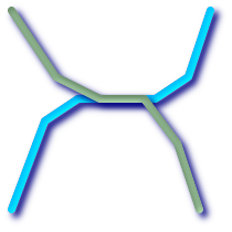
A
MULTILINESTRING
is
simple
only if all of its elements are simple and the only intersection between
any two elements occurs at
POINT
s that are on the
boundaries of both elements.

(e) |

(f) |

(g) |
|
(e)
and
(f)
are simple
|
By definition, a
POLYGON
is always
simple
. It is
valid
if no two
rings in the boundary (made up of an exterior ring and interior rings)
cross. The boundary of a
POLYGON
may intersect at a
POINT
but only as a tangent (i.e. not on a line).
A
POLYGON
may not have cut lines or spikes and the
interior rings must be contained entirely within the exterior ring.

(h) |

(i) |

(j) |

(k) |

(l) |

(m) |
|
(h)
and
(i)
are valid
|
A
MULTIPOLYGON
is
valid
if and only if all of its elements are valid and the interiors of no two
elements intersect. The boundaries of any two elements may touch, but
only at a finite number of
POINT
s.

(n) |

(o) |

(p) |
|
(n)
and
(o)
are not valid
|
Most of the functions implemented by the GEOS library rely on the assumption that your geometries are valid as specified by the OpenGIS Simple Feature Specification. To check simplicity or validity of geometries you can use the ST_IsSimple() and ST_IsValid()
-- Typically, it doesn't make sense to check
-- for validity on linear features since it will always return TRUE.
-- But in this example, PostGIS extends the definition of the OGC IsValid
-- by returning false if a LineString has less than 2 *distinct* vertices.
gisdb=# SELECT
   ST_IsValid('LINESTRING(0 0, 1 1)'),
   ST_IsValid('LINESTRING(0 0, 0 0, 0 0)');

 st_isvalid | st_isvalid
------------+-----------
      t     |     f
By default, PostGIS does not apply this validity check on geometry input, because testing for validity needs lots of CPU time for complex geometries, especially polygons. If you do not trust your data sources, you can manually enforce such a check to your tables by adding a check constraint:
ALTER TABLE mytable
  ADD CONSTRAINT geometry_valid_check
	CHECK (ST_IsValid(the_geom));
If you encounter any strange error messages such as "GEOS Intersection() threw an error!" when calling PostGIS functions with valid input geometries, you likely found an error in either PostGIS or one of the libraries it uses, and you should contact the PostGIS developers. The same is true if a PostGIS function returns an invalid geometry for valid input.
|
|
|
|
Strictly compliant OGC geometries cannot have Z or M values. The ST_IsValid() function won't consider higher dimensioned geometries invalid! Invocations of AddGeometryColumn() will add a constraint checking geometry dimensions, so it is enough to specify 2 there. |
It is sometimes the case that the typical spatial predicates ( ST_Intersects , ST_Contains , ST_Crosses , ST_Touches , ...) are insufficient in and of themselves to adequately provide that desired spatial filter.
For example, consider a linear
dataset representing a road network. It may be the task of a
GIS analyst to identify all road segments that cross
each other, not at a point, but on a line, perhaps invalidating
some business rule. In this case,
ST_Crosses
does not
adequately provide the necessary spatial filter since, for
linear features, it returns
One two-step solution
might be to first perform the actual intersection
(
ST_Intersection
) of pairs of road segments that spatially
intersect (
ST_Intersects
), and then compare the intersection's
ST_GeometryType
with '
A more elegant / faster solution may indeed be desirable. |
|

A second [theoretical] example may be that of a GIS analyst trying to locate all wharfs or docks that intersect a lake's boundary on a line and where only one end of the wharf is up on shore. In other words, where a wharf is within, but not completely within a lake, intersecting the boundary of a lake on a line, and where the wharf's endpoints are both completely within and on the boundary of the lake. The analyst may need to use a combination of spatial predicates to isolate the sought after features:
|
So enters the Dimensionally Extended 9 Intersection Model, or DE-9IM for short.
According to the OpenGIS Simple Features Implementation Specification for SQL , "the basic approach to comparing two geometries is to make pair-wise tests of the intersections between the Interiors, Boundaries and Exteriors of the two geometries and to classify the relationship between the two geometries based on the entries in the resulting 'intersection' matrix."
- Boundary
-
The boundary of a geometry is the set of geometries of the next lower dimension. For
POINTs, which have a dimension of 0, the boundary is the empty set. The boundary of aLINESTRINGare the two endpoints. ForPOLYGONs, the boundary is the linework that make up the exterior and interior rings. - Interior
-
The interior of a geometry are those points of a geometry that are left when the boundary is removed. For
POINTs, the interior is thePOINTitself. The interior of aLINESTRINGare the set of real points between the endpoints. ForPOLYGONs, the interior is the areal surface inside the polygon. - Exterior
-
The exterior of a geometry is the universe, an areal surface, not on the interior or boundary of the geometry.
Given geometry a , where the I(a) , B(a) , and E(a) are the Interior , Boundary , and Exterior of a, the mathematical representation of the matrix is:
| Interior | Boundary | Exterior | |
|---|---|---|---|
| Interior | dim( I(a) ∩ I(b) ) | dim( I(a) ∩ B(b) ) | dim( I(a) ∩ E(b) ) |
| Boundary | dim( B(a) ∩ I(b) ) | dim( B(a) ∩ B(b) ) | dim( B(a) ∩ E(b) ) |
| Exterior | dim( E(a) ∩ I(b) ) | dim( E(a) ∩ B(b) ) | dim( E(a) ∩ E(b) ) |
Where
dim(a)
is the dimension of
a
as specified by
ST_Dimension
but has the domain of
{0,1,2,T,F,*}
-
0=> point -
1=> line -
2=> area -
T=>{0,1,2} -
F=> empty set -
*=> don't care
Visually, for two overlapping polygonal geometries, this looks like:
|
||||||||||||||||||
|
|


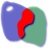
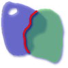

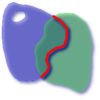
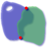


Read from left to right and from top to bottom, the dimensional matrix is represented, ' 212101212 '.
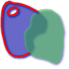
A relate matrix that would therefore represent our first example of two lines that intersect on a line would be: ' 1*1***1** '
-- Identify road segments that cross on a line
SELECT a.id
FROM roads a, roads b
WHERE a.id != b.id
AND a.geom && b.geom
AND ST_Relate(a.geom, b.geom, '1*1***1**');
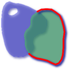
A relate matrix that represents the second example of wharfs partly on the lake's shoreline would be ' 102101FF2 '
-- Identify wharfs partly on a lake's shoreline
SELECT a.lake_id, b.wharf_id
FROM lakes a, wharfs b
WHERE a.geom && b.geom
AND ST_Relate(a.geom, b.geom, '102101FF2');
For more information or reading, see:
-
OpenGIS Simple Features Implementation Specification for SQL (version 1.1, section 2.1.13.2)
-
Encyclopedia of GIS By Hui Xiong
Once you have created a spatial table, you are ready to upload GIS data to the database. Currently, there are two ways to get data into a PostGIS/PostgreSQL database: using formatted SQL statements or using the Shape file loader/dumper.
If you can convert your data to a text representation, then using formatted SQL might be the easiest way to get your data into PostGIS. As with Oracle and other SQL databases, data can be bulk loaded by piping a large text file full of SQL "INSERT" statements into the SQL terminal monitor.
A data upload file (
roads.sql
for example)
might look like this:
BEGIN;
INSERT INTO roads (road_id, roads_geom, road_name)
  VALUES (1,'LINESTRING(191232 243118,191108 243242)','Jeff Rd');
INSERT INTO roads (road_id, roads_geom, road_name)
  VALUES (2,'LINESTRING(189141 244158,189265 244817)','Geordie Rd');
INSERT INTO roads (road_id, roads_geom, road_name)
  VALUES (3,'LINESTRING(192783 228138,192612 229814)','Paul St');
INSERT INTO roads (road_id, roads_geom, road_name)
  VALUES (4,'LINESTRING(189412 252431,189631 259122)','Graeme Ave');
INSERT INTO roads (road_id, roads_geom, road_name)
  VALUES (5,'LINESTRING(190131 224148,190871 228134)','Phil Tce');
INSERT INTO roads (road_id, roads_geom, road_name)
  VALUES (6,'LINESTRING(198231 263418,198213 268322)','Dave Cres');
COMMIT;
The data file can be piped into PostgreSQL very easily using the "psql" SQL terminal monitor:
psql -d [database] -f roads.sql
The
shp2pgsql
data loader converts ESRI Shape files into SQL suitable for
insertion into a PostGIS/PostgreSQL database either in geometry or geography format. The loader has several operating modes
distinguished by command line flags:
In addition to the shp2pgsql command-line loader, there is an
shp2pgsql-gui
graphical interface with most
of the options as the command-line loader, but may be easier to use for one-off non-scripted loading or if you are new to PostGIS.
It can also be configured as a plugin to PgAdminIII.
- (c|a|d|p) These are mutually exclusive options:
-
- -c
-
Creates a new table and populates it from the shapefile. This is the default mode.
- -a
-
Appends data from the Shape file into the database table. Note that to use this option to load multiple files, the files must have the same attributes and same data types.
- -d
-
Drops the database table before creating a new table with the data in the Shape file.
- -p
-
Only produces the table creation SQL code, without adding any actual data. This can be used if you need to completely separate the table creation and data loading steps.
- -?
-
Display help screen.
- -D
-
Use the PostgreSQL "dump" format for the output data. This can be combined with -a, -c and -d. It is much faster to load than the default "insert" SQL format. Use this for very large data sets.
- -s [<FROM_SRID%gt;:]<SRID>
-
Creates and populates the geometry tables with the specified SRID. Optionally specifies that the input shapefile uses the given FROM_SRID, in which case the geometries will be reprojected to the target SRID. FROM_SRID cannot be specified with -D.
- -k
-
Keep identifiers' case (column, schema and attributes). Note that attributes in Shapefile are all UPPERCASE.
- -i
-
Coerce all integers to standard 32-bit integers, do not create 64-bit bigints, even if the DBF header signature appears to warrant it.
- -I
-
Create a GiST index on the geometry column.
- -m
-
-m
a_file_nameSpecify a file containing a set of mappings of (long) column names to 10 character DBF column names. The content of the file is one or more lines of two names separated by white space and no trailing or leading space. For example:COLUMNNAME DBFFIELD1 AVERYLONGCOLUMNNAME DBFFIELD2
- -S
-
Generate simple geometries instead of MULTI geometries. Will only succeed if all the geometries are actually single (I.E. a MULTIPOLYGON with a single shell, or or a MULTIPOINT with a single vertex).
- -t <dimensionality>
-
Force the output geometry to have the specified dimensionality. Use the following strings to indicate the dimensionality: 2D, 3DZ, 3DM, 4D.
If the input has fewer dimensions that specified, the output will have those dimensions filled in with zeroes. If the input has more dimensions that specified, the unwanted dimensions will be stripped.
- -w
-
Output WKT format, instead of WKB. Note that this can introduce coordinate drifts due to loss of precision.
- -e
-
Execute each statement on its own, without using a transaction. This allows loading of the majority of good data when there are some bad geometries that generate errors. Note that this cannot be used with the -D flag as the "dump" format always uses a transaction.
- -W <encoding>
-
Specify encoding of the input data (dbf file). When used, all attributes of the dbf are converted from the specified encoding to UTF8. The resulting SQL output will contain a
SET CLIENT_ENCODING to UTF8command, so that the backend will be able to reconvert from UTF8 to whatever encoding the database is configured to use internally. - -N <policy>
-
NULL geometries handling policy (insert*,skip,abort)
- -n
-
-n Only import DBF file. If your data has no corresponding shapefile, it will automatically switch to this mode and load just the dbf. So setting this flag is only needed if you have a full shapefile set, and you only want the attribute data and no geometry.
- -G
-
Use geography type instead of geometry (requires lon/lat data) in WGS84 long lat (SRID=4326)
- -T <tablespace>
-
Specify the tablespace for the new table. Indexes will still use the default tablespace unless the -X parameter is also used. The PostgreSQL documentation has a good description on when to use custom tablespaces.
- -X <tablespace>
-
Specify the tablespace for the new table's indexes. This applies to the primary key index, and the GIST spatial index if -I is also used.
An example session using the loader to create an input file and uploading it might look like this:
# shp2pgsql -c -D -s 4269 -i -I shaperoads.shp myschema.roadstable > roads.sql
# psql -d roadsdb -f roads.sql
A conversion and upload can be done all in one step using UNIX pipes:
# shp2pgsql shaperoads.shp myschema.roadstable | psql -d roadsdb
Data can be extracted from the database using either SQL or the Shape file loader/dumper. In the section on SQL we will discuss some of the operators available to do comparisons and queries on spatial tables.
The most straightforward means of pulling data out of the database is to use a SQL select query to reduce the number of RECORDS and COLUMNS returned and dump the resulting columns into a parsable text file:
db=# SELECT road_id, ST_AsText(road_geom) AS geom, road_name FROM roads;

road_id | geom                                    | road_name
--------+-----------------------------------------+-----------
	  1 | LINESTRING(191232 243118,191108 243242) | Jeff Rd
	  2 | LINESTRING(189141 244158,189265 244817) | Geordie Rd
	  3 | LINESTRING(192783 228138,192612 229814) | Paul St
	  4 | LINESTRING(189412 252431,189631 259122) | Graeme Ave
	  5 | LINESTRING(190131 224148,190871 228134) | Phil Tce
	  6 | LINESTRING(198231 263418,198213 268322) | Dave Cres
	  7 | LINESTRING(218421 284121,224123 241231) | Chris Way
(6 rows)
However, there will be times when some kind of restriction is necessary to cut down the number of fields returned. In the case of attribute-based restrictions, just use the same SQL syntax as normal with a non-spatial table. In the case of spatial restrictions, the following operators are available/useful:
- ST_Intersects
-
This function tells whether two geometries share any space.
- =
-
This tests whether two geometries are geometrically identical. For example, if 'POLYGON((0 0,1 1,1 0,0 0))' is the same as 'POLYGON((0 0,1 1,1 0,0 0))' (it is).
Note: before PostGIS 2.4 this compared only boxes of geometries.
Next, you can use these operators in queries. Note that when specifying geometries and boxes on the SQL command line, you must explicitly turn the string representations into geometries function. The 312 is a fictitious spatial reference system that matches our data. So, for example:
SELECT road_id, road_name
  FROM roads
  WHERE roads_geom='SRID=312;LINESTRING(191232 243118,191108 243242)'::geometry;
The above query would return the single record from the "ROADS_GEOM" table in which the geometry was equal to that value.
To check whether some of the roads passes in the area defined by a polygon:
SELECT road_id, road_name
FROM roads
WHERE ST_Intersects(roads_geom, 'SRID=312;POLYGON((...))');
The most common spatial query will probably be a "frame-based" query, used by client software, like data browsers and web mappers, to grab a "map frame" worth of data for display.
When using the "&&" operator, you can specify either a BOX3D as the comparison feature or a GEOMETRY. When you specify a GEOMETRY, however, its bounding box will be used for the comparison.
Using a "BOX3D" object for the frame, such a query looks like this:
SELECT ST_AsText(roads_geom) AS geom
FROM roads
WHERE
  roads_geom && ST_MakeEnvelope(191232, 243117,191232, 243119,312);
Note the use of the SRID 312, to specify the projection of the envelope.
The
pgsql2shp
table dumper connects directly
to the database and converts a table (possibly defined by a query) into
a shape file. The basic syntax is:
pgsql2shp [<options>] <database> [<schema>.]<table>
pgsql2shp [<options>] <database> <query>
The commandline options are:
- -f <filename>
-
Write the output to a particular filename.
- -h <host>
-
The database host to connect to.
- -p <port>
-
The port to connect to on the database host.
- -P <password>
-
The password to use when connecting to the database.
- -u <user>
-
The username to use when connecting to the database.
- -g <geometry column>
-
In the case of tables with multiple geometry columns, the geometry column to use when writing the shape file.
- -b
-
Use a binary cursor. This will make the operation faster, but will not work if any NON-geometry attribute in the table lacks a cast to text.
- -r
-
Raw mode. Do not drop the
gidfield, or escape column names. -
-m
filename -
Remap identifiers to ten character names. The content of the file is lines of two symbols separated by a single white space and no trailing or leading space: VERYLONGSYMBOL SHORTONE ANOTHERVERYLONGSYMBOL SHORTER etc.
Indexes are what make using a spatial database for large data sets possible. Without indexing, any search for a feature would require a "sequential scan" of every record in the database. Indexing speeds up searching by organizing the data into a search tree which can be quickly traversed to find a particular record. PostgreSQL supports three kinds of indexes by default: B-Tree indexes, SP-GiST and GiST indexes.
-
B-Trees are used for data which can be sorted along one axis; for example, numbers, letters, dates. Spatial data can be sorted along a space-filling curve, Z-order curve or Hilbert curve. This representation however does not allow speeding up common operations.
-
GiST (Generalized Search Trees) indexes break up data into "things to one side", "things which overlap", "things which are inside" and can be used on a wide range of data-types, including GIS data. PostGIS uses an R-Tree index implemented on top of GiST to index GIS data.
GiST stands for "Generalized Search Tree" and is a generic form of indexing. In addition to GIS indexing, GiST is used to speed up searches on all kinds of irregular data structures (integer arrays, spectral data, etc) which are not amenable to normal B-Tree indexing.
Once a GIS data table exceeds a few thousand rows, you will want to build an index to speed up spatial searches of the data (unless all your searches are based on attributes, in which case you'll want to build a normal index on the attribute fields).
The syntax for building a GiST index on a "geometry" column is as follows:
CREATE INDEX [indexname] ON [tablename] USING GIST ( [geometryfield] );
The above syntax will always build a 2D-index. To get the an n-dimensional index for the geometry type, you can create one using this syntax:
CREATE INDEX [indexname] ON [tablename] USING GIST ([geometryfield] gist_geometry_ops_nd);
Building a spatial index is a computationally intensive exercise. It also blocks write access to your table for the time it creates, so on a production system you may want to do in in a slower CONCURRENTLY-aware way:
CREATE INDEX CONCURRENTLY [indexname] ON [tablename] USING GIST ( [geometryfield] );
After building an index, it is sometimes helpful to force PostgreSQL to collect table statistics, which are used to optimize query plans:
VACUUM ANALYZE [table_name] [(column_name)];
BRIN stands for "Block Range Index" and is a generic form of indexing that has been introduced in PostgreSQL 9.5. BRIN is a lossy kind of index, and its main usage is to provide a compromise for both read and write performance. Its primary goal is to handle very large tables for which some of the columns have some natural correlation with their physical location within the table. In addition to GIS indexing, BRIN is used to speed up searches on various kinds of regular or irregular data structures (integer, arrays etc).
Once a GIS data table exceeds a few thousand rows, you will want to build an index to speed up spatial searches of the data (unless all your searches are based on attributes, in which case you'll want to build a normal index on the attribute fields). GiST indexes are really performant as long as their size doesn't exceed the amount of RAM available for the database, and as long as you can afford the storage size, and the penalty in write workload. Otherwise, BRIN index can be considered as an alternative.
The idea of a BRIN index is to store only the bouding box englobing all the geometries contained in all the rows in a set of table blocks, called a range. Obviously, this indexing method will only be efficient if the data is physically ordered in a way where the resulting bouding boxes for block ranges will be mutually exclusive. The resulting index will be really small, but will be less efficient than a GiST index in many cases.
Building a BRIN index is way less intensive than building a GiST index. It's quite common to build a BRIN index in more than ten time less than a GiST index would have required. As a BRIN index only store one bouding box for one to many table blocks, it's pretty common to consume up to a thousand time less disk space for this kind of indexes.
You can choose the number of blocks to summarize in a range. If you decrease this number, the index will be bigger but will probably help to get better performance.
The syntax for building a BRIN index on a "geometry" column is as follows:
CREATE INDEX [indexname] ON [tablename] USING BRIN ( [geometryfield] );
The above syntax will always build a 2D-index. To get a 3D-dimensional index, you can create one using this syntax
CREATE INDEX [indexname] ON [tablename] USING BRIN ([geometryfield] brin_geometry_inclusion_ops_3d);
You can also get a 4D-dimensional index using the 4D operator class
CREATE INDEX [indexname] ON [tablename] USING BRIN ([geometryfield] brin_geometry_inclusion_ops_4d);
These above syntaxes will use the default number or block in a range, which is 128. To specify the number of blocks you want to summarise in a range, you can create one using this syntax
CREATE INDEX [indexname] ON [tablename] USING BRIN ( [geometryfield] ) WITH (pages_per_range = [number]);
Also, keep in mind that a BRIN index will only store one index value for a large number of rows. If your table stores geometries with a mixed number of dimensions, it's likely that the resulting index will have poor performance. You can avoid this drop of performance by choosing the operator class whith the least number of dimensions of the stored geometries
Also the "geography" datatype is supported for BRIN indexing. The syntax for building a BRIN index on a "geography" column is as follows:
CREATE INDEX [indexname] ON [tablename] USING BRIN ( [geographyfield] );
The above syntax will always build a 2D-index for geospatial objects on the spheroid.
Currently, just the "inclusion support" is considered here, meaning
that just
&&
,
~
and
@
operators can be used for the 2D cases (both for
"geometry" and for "geography"), and just the
&&&
operator can be used for the 3D geometries. There is no support
for kNN searches at the moment.
SP-GiST stands for "Space-Partitioned Generalized Search Tree" and is a generic form of indexing that supports partitioned search trees, such as quad-trees, k-d trees, and radix trees (tries). The common feature of these data structures is that they repeatedly divide the search space into partitions that need not be of equal size. In addition to GIS indexing, SP-GiST is used to speed up searches on many kinds of data, such as phone routing, ip routing, substring search, etc.
As it is the case for GiST indexes, SP-GiST indexes are lossy, in the sense that they store the bounding box englobing the spatial objects. SP-GiST indexes can be considered as an alternative to GiST indexes. The performance tests reveal that SP-GiST indexes are especially beneficial when there are many overlapping objects, that is, with so-called “spaghetti data”.
Once a GIS data table exceeds a few thousand rows, an SP-GiST index may be used to speed up spatial searches of the data. The syntax for building an SP-GiST index on a "geometry" column is as follows:
CREATE INDEX [indexname] ON [tablename] USING SPGIST ( [geometryfield] );
The above syntax will build a 2-dimensional index. A 3-dimensional index for the geometry type can be created using the 3D operator class:
CREATE INDEX [indexname] ON [tablename] USING SPGIST ([geometryfield] spgist_geometry_ops_3d);
Building a spatial index is a computationally intensive operation. It also blocks write access to your table for the time it creates, so on a production system you may want to do in in a slower CONCURRENTLY-aware way:
CREATE INDEX CONCURRENTLY [indexname] ON [tablename] USING SPGIST ( [geometryfield] );
After building an index, it is sometimes helpful to force PostgreSQL to collect table statistics, which are used to optimize query plans:
VACUUM ANALYZE [table_name] [(column_name)];
An SP-GiST index can accelerate queries involving the following operators:
-
<<, &<, &>, >>, <<|, &<|, |&>, |>>, &&, @>, <@, and ~=, for 2-dimensional indexes,
-
&/&, ~==, @>>, and <<@, for 3-dimensional indexes.
There is no support for kNN searches at the moment.
Ordinarily, indexes invisibly speed up data access: once the index is built, the query planner transparently decides when to use index information to speed up a query plan. Unfortunately, the PostgreSQL query planner sometimes does not optimize the use of GiST indexes well, so sometimes searches which should use a spatial index instead may perform a sequential scan of the whole table.
If you find your spatial indexes are not being used (or your attribute indexes, for that matter) there are a couple things you can do:
-
Firstly, read query plan and check your query actually tries to compute the thing you need. A runaway JOIN condition, either forgotten or to the wrong table, can unexpectedly bring you all of your table multiple times. To get query plan, add EXPLAIN keyword in front of your query.
-
Second, make sure statistics are gathered about the number and distributions of values in a table, to provide the query planner with better information to make decisions around index usage. VACUUM ANALYZE will compute both.
You should regularly vacuum your databases anyways - many PostgreSQL DBAs have VACUUM run as an off-peak cron job on a regular basis.
-
If vacuuming does not help, you can temporarily force the planner to use the index information by using the set enable_seqscan to off; command. This way you can check whether planner is at all capable to generate an index accelerated query plan for your query. You should only use this command only for debug: generally speaking, the planner knows better than you do about when to use indexes. Once you have run your query, do not forget to set
ENABLE_SEQSCANback on, so that other queries will utilize the planner as normal. -
If set enable_seqscan to off; helps your query to run, your Postgres is likely not tuned for your hardware. If you find the planner wrong about the cost of sequential vs index scans try reducing the value of
random_page_costin postgresql.conf or using set random_page_cost to 1.1; . Default value for the parameter is 4, try setting it to 1 (on SSD) or 2 (on fast magnetic disks). Decreasing the value makes the planner more inclined of using Index scans. -
If set enable_seqscan to off; does not help your query, it may happen you use a construction Postgres is not yet able to untangle. A subquery with inline select is one example - you need to rewrite it to the form planner can optimize, say, a LATERAL JOIN.
The raison d'etre of spatial database functionality is performing queries inside the database which would ordinarily require desktop GIS functionality. Using PostGIS effectively requires knowing what spatial functions are available, and ensuring that appropriate indexes are in place to provide good performance. The SRID of 312 used in these examples is purely for demonstration. You should be using a REAL SRID listed in the the spatial_ref_sys table and one that matches the projection of your data. If your data has no spatial reference system specified, you should be THINKING very thoughtfully why it doesn't and maybe it should.
If your reason is because you are modeling something that doesn't have a geographic spatial reference system defined such as the internals of a molecule or the floorplan of a not yet built amusement park then that's fine. If the location of the amusement park has been planned however, then it would make sense to use a suitable planar coordinate system for that location if nothing more than to ensure the amusement part is not trespassing on already existing structures.
Even in the case where you are planning a Mars expedition to transport the human race in the event of a nuclear holocaust
and you want to map out the Mars planet for rehabitation, you can use a non-earthly coordinate system such as
Mars 2000
make one up and insert it in the
spatial_ref_sys
table. Though this Mars coordinate system is a non-planar one (it's in degrees spheroidal),
you can use it with the geography type to have your length and proximity measurements in meters instead of degrees.
When constructing a query it is important to remember that only
the bounding-box-based operators such as && can take advantage
of the GiST spatial index. Functions such as
ST_Distance()
cannot use the index to optimize their
operation. For example, the following query would be quite slow on a
large table:
SELECT the_geom
FROM geom_table
WHERE ST_Distance(the_geom, 'SRID=312;POINT(100000 200000)') < 100
This query is selecting all the geometries in geom_table which are
within 100 units of the point (100000, 200000). It will be slow because
it is calculating the distance between each point in the table and our
specified point, ie. one
ST_Distance()
calculation
for each row in the table. We can avoid this by using the single step
index accelerated function ST_DWithin to reduce the number of distance
calculations required:
SELECT the_geom
FROM geom_table
WHERE ST_DWithin(the_geom, 'SRID=312;POINT(100000 200000)', 100)
This query selects the same geometries, but it does it in a more
efficient way. Assuming there is a GiST index on the_geom, the query
planner will recognize that it can use the index to reduce the number of
rows before calculating the result of the
ST_Distance()
function. Notice that the
ST_MakeEnvelope
geometry which is
used in the && operation is a 200 unit square box centered on
the original point - this is our "query box". The && operator
uses the index to quickly reduce the result set down to only those
geometries which have bounding boxes that overlap the "query box".
Assuming that our query box is much smaller than the extents of the
entire geometry table, this will drastically reduce the number of
distance calculations that need to be done.
The examples in this section will make use of two tables, a table
of linear roads, and a table of polygonal municipality boundaries. The
table definitions for the
bc_roads
table is:
Column      | Type              | Description
------------+-------------------+-------------------
gid         | integer           | Unique ID
name        | character varying | Road Name
the_geom    | geometry          | Location Geometry (Linestring)
The table definition for the
bc_municipality
table is:
Column     | Type              | Description
-----------+-------------------+-------------------
gid        | integer           | Unique ID
code       | integer           | Unique ID
name       | character varying | City / Town Name
the_geom   | geometry          | Location Geometry (Polygon)
- 4.7.2.1. What is the total length of all roads, expressed in kilometers?
- 4.7.2.2. How large is the city of Prince George, in hectares?
- 4.7.2.3. What is the largest municipality in the province, by area?
- 4.7.2.4. What is the length of roads fully contained within each municipality?
- 4.7.2.5. Create a new table with all the roads within the city of Prince George.
- 4.7.2.6. What is the length in kilometers of "Douglas St" in Victoria?
- 4.7.2.7. What is the largest municipality polygon that has a hole?