Chapter 4. PostGIS Usage
- 4.1. Data Management
- 4.2. Spatial Queries
- 4.3. Performance Tips
- 4.4. Building Applications
- 4.5. Raster Data Management, Queries, and Applications
- 4.6. Topology
-
- 4.6.1. Topology Types
- 4.6.2. Topology Domains
- 4.6.3. Topology and TopoGeometry Management
- 4.6.4. Topology Statistics Management
- 4.6.5. Topology Constructors
- 4.6.6. Topology Editors
- 4.6.7. Topology Accessors
- 4.6.8. Topology Processing
- 4.6.9. TopoGeometry Constructors
- 4.6.10. TopoGeometry Editors
- 4.6.11. TopoGeometry Accessors
- 4.6.12. TopoGeometry Outputs
- 4.6.13. Topology Spatial Relationships
- 4.7. Address Standardizer
- 4.8. PostGIS Extras
The GIS objects supported by PostGIS are a superset of the "Simple Features" standard defined by the OpenGIS Consortium (OGC). PostGIS supports all the objects and functions specified in the OGC "Simple Features for SQL" specification (SFS).
PostGIS extends the standard with support for embedded SRID information.
The OpenGIS specification defines two standard ways of expressing spatial objects: the Well-Known Text (WKT) form and the Well-Known Binary (WKB) form. Both WKT and WKB include information about the type of the object and the coordinates which form the object.
Examples of the text representations (WKT) of the spatial objects of the features are as follows:
-
POINT(0 0)
-
POINT Z (0 0 0)
-
POINT ZM (0 0 0 0)
-
LINESTRING(0 0,1 1,1 2)
-
POLYGON((0 0,4 0,4 4,0 4,0 0),(1 1, 2 1, 2 2, 1 2,1 1))
-
MULTIPOINT((0 0),(1 2))
-
MULTIPOINT Z ((0 0 0),(1 2 3))
-
MULTILINESTRING((0 0,1 1,1 2),(2 3,3 2,5 4))
-
MULTIPOLYGON(((0 0,4 0,4 4,0 4,0 0),(1 1,2 1,2 2,1 2,1 1)), ((-1 -1,-1 -2,-2 -2,-2 -1,-1 -1)))
-
GEOMETRYCOLLECTION(POINT(2 3),LINESTRING(2 3,3 4))
The OpenGIS specification also requires that the internal storage format of spatial objects include a spatial referencing system identifier (SRID). The SRID is required when creating spatial objects for insertion into the database.
Input/Output of these formats are available using the following interfaces:
bytea WKB = ST_AsBinary(geometry);
text WKT = ST_AsText(geometry);
geometry = ST_GeomFromWKB(bytea WKB, SRID);
geometry = ST_GeometryFromText(text WKT, SRID);
For example, a valid insert statement to create and insert an OGC spatial object would be:
INSERT INTO geotable ( the_geom, the_name )
  VALUES ( ST_GeomFromText('POINT(-126.4 45.32)', 312), 'A Place');
First OpenGIS specifications (prior to 1.2.0) only support 2D geometries, and the associated SRID is *never* embedded in the input/output representations.
Even though the last OpenGIS specification 1.2.1 supports 3DM and 3DZ coordinates specifing ZM qualifiers, it does not include yet the associated SRID in the input/output representations.
PostGIS extended formats add 3DM, 3DZ, 4D coordinates support and embedded SRID information. However, PostGIS EWKB/EWKT outputs have several peculiarities:
-
For 3DZ geometries they will drop the Z qualifier:
OpenGIS: POINT Z (1 2 3)
EWKB/EWKT: POINT(1 2 3)
-
For 3DM geometries they will keep the M qualifier:
OpenGIS: POINT M (1 2 3)
EWKB/EWKT: POINTM(1 2 3)
-
For 4D geometries they will drop the ZM qualifiers:
OpenGIS: POINT ZM (1 2 3 4)
EWKB/EWKT: POINT(1 2 3 4)
By doing this, PostGIS EWKB/EWKT avoids over-specifying dimensionality and a whole categories of potential errors that ISO admits, e.g.:
-
POINT ZM (1 1)
-
POINT ZM (1 1 1)
-
POINT (1 1 1 1)
![[Caution]](images/caution.png)
|
|
|
PostGIS extended formats are currently superset of the OGC one (every valid WKB/WKT is a valid EWKB/EWKT) but this might vary in the future, specifically if OGC comes out with a new format conflicting with our extensions. Thus you SHOULD NOT rely on this feature! |
Examples of the text representations (EWKT) of the extended spatial objects of the features are as follows.
-
POINT(0 0 0) -- XYZ
-
SRID=32632;POINT(0 0) -- XY with SRID
-
POINTM(0 0 0) -- XYM
-
POINT(0 0 0 0) -- XYZM
-
SRID=4326;MULTIPOINTM(0 0 0,1 2 1) -- XYM with SRID
-
MULTILINESTRING((0 0 0,1 1 0,1 2 1),(2 3 1,3 2 1,5 4 1))
-
POLYGON((0 0 0,4 0 0,4 4 0,0 4 0,0 0 0),(1 1 0,2 1 0,2 2 0,1 2 0,1 1 0))
-
MULTIPOLYGON(((0 0 0,4 0 0,4 4 0,0 4 0,0 0 0),(1 1 0,2 1 0,2 2 0,1 2 0,1 1 0)),((-1 -1 0,-1 -2 0,-2 -2 0,-2 -1 0,-1 -1 0)))
-
GEOMETRYCOLLECTIONM( POINTM(2 3 9), LINESTRINGM(2 3 4, 3 4 5) )
-
MULTICURVE( (0 0, 5 5), CIRCULARSTRING(4 0, 4 4, 8 4) )
-
POLYHEDRALSURFACE( ((0 0 0, 0 0 1, 0 1 1, 0 1 0, 0 0 0)), ((0 0 0, 0 1 0, 1 1 0, 1 0 0, 0 0 0)), ((0 0 0, 1 0 0, 1 0 1, 0 0 1, 0 0 0)), ((1 1 0, 1 1 1, 1 0 1, 1 0 0, 1 1 0)), ((0 1 0, 0 1 1, 1 1 1, 1 1 0, 0 1 0)), ((0 0 1, 1 0 1, 1 1 1, 0 1 1, 0 0 1)) )
-
TRIANGLE ((0 0, 0 9, 9 0, 0 0))
-
TIN( ((0 0 0, 0 0 1, 0 1 0, 0 0 0)), ((0 0 0, 0 1 0, 1 1 0, 0 0 0)) )
Conversion between these formats is available using the following interfaces:
bytea EWKB = ST_AsEWKB(geometry);
text EWKT = ST_AsEWKT(geometry);
geometry = ST_GeomFromEWKB(bytea EWKB);
geometry = ST_GeomFromEWKT(text EWKT);
For example, a valid insert statement to create and insert a PostGIS spatial object would be:
INSERT INTO geotable ( the_geom, the_name )
  VALUES ( ST_GeomFromEWKT('SRID=312;POINTM(-126.4 45.32 15)'), 'A Place' )
The "canonical forms" of a PostgreSQL type are the representations you get with a simple query (without any function call) and the one which is guaranteed to be accepted with a simple insert, update or copy. For the PostGIS 'geometry' type these are:
- Output
  - binary: EWKB
	ascii: HEXEWKB (EWKB in hex form)
- Input
  - binary: EWKB
	ascii: HEXEWKB|EWKT
For example this statement reads EWKT and returns HEXEWKB in the process of canonical ascii input/output:
=# SELECT 'SRID=4;POINT(0 0)'::geometry;

geometry
----------------------------------------------------
01010000200400000000000000000000000000000000000000
(1 row)
The SQL Multimedia Applications Spatial specification extends the simple features for SQL spec by defining a number of circularly interpolated curves.
The SQL-MM definitions include 3DM, 3DZ and 4D coordinates, but do not allow the embedding of SRID information.
The Well-Known Text extensions are not yet fully supported. Examples of some simple curved geometries are shown below:
-
CIRCULARSTRING(0 0, 1 1, 1 0)
CIRCULARSTRING(0 0, 4 0, 4 4, 0 4, 0 0)
The CIRCULARSTRING is the basic curve type, similar to a LINESTRING in the linear world. A single segment required three points, the start and end points (first and third) and any other point on the arc. The exception to this is for a closed circle, where the start and end points are the same. In this case the second point MUST be the center of the arc, ie the opposite side of the circle. To chain arcs together, the last point of the previous arc becomes the first point of the next arc, just like in LINESTRING. This means that a valid circular string must have an odd number of points greater than 1.
-
COMPOUNDCURVE(CIRCULARSTRING(0 0, 1 1, 1 0),(1 0, 0 1))
A compound curve is a single, continuous curve that has both curved (circular) segments and linear segments. That means that in addition to having well-formed components, the end point of every component (except the last) must be coincident with the start point of the following component.
-
CURVEPOLYGON(CIRCULARSTRING(0 0, 4 0, 4 4, 0 4, 0 0),(1 1, 3 3, 3 1, 1 1))
Example compound curve in a curve polygon: CURVEPOLYGON(COMPOUNDCURVE(CIRCULARSTRING(0 0,2 0, 2 1, 2 3, 4 3),(4 3, 4 5, 1 4, 0 0)), CIRCULARSTRING(1.7 1, 1.4 0.4, 1.6 0.4, 1.6 0.5, 1.7 1) )
A CURVEPOLYGON is just like a polygon, with an outer ring and zero or more inner rings. The difference is that a ring can take the form of a circular string, linear string or compound string.
As of PostGIS 1.4 PostGIS supports compound curves in a curve polygon.
-
MULTICURVE((0 0, 5 5),CIRCULARSTRING(4 0, 4 4, 8 4))
The MULTICURVE is a collection of curves, which can include linear strings, circular strings or compound strings.
-
MULTISURFACE(CURVEPOLYGON(CIRCULARSTRING(0 0, 4 0, 4 4, 0 4, 0 0),(1 1, 3 3, 3 1, 1 1)),((10 10, 14 12, 11 10, 10 10),(11 11, 11.5 11, 11 11.5, 11 11)))
This is a collection of surfaces, which can be (linear) polygons or curve polygons.
![[Note]](images/note.png)
|
|
|
All floating point comparisons within the SQL-MM implementation are performed to a specified tolerance, currently 1E-8. |
The geography type provides native support for spatial features represented on "geographic" coordinates (sometimes called "geodetic" coordinates, or "lat/lon", or "lon/lat"). Geographic coordinates are spherical coordinates expressed in angular units (degrees).
The basis for the PostGIS geometry type is a plane. The shortest path between two points on the plane is a straight line. That means calculations on geometries (areas, distances, lengths, intersections, etc) can be calculated using cartesian mathematics and straight line vectors.
The basis for the PostGIS geographic type is a sphere. The shortest path between two points on the sphere is a great circle arc. That means that calculations on geographies (areas, distances, lengths, intersections, etc) must be calculated on the sphere, using more complicated mathematics. For more accurate measurements, the calculations must take the actual spheroidal shape of the world into account.
Because the underlying mathematics is much more complicated, there are fewer functions defined for the geography type than for the geometry type. Over time, as new algorithms are added, the capabilities of the geography type will expand.
It uses a data type called
geography
. None of the GEOS functions support the
geography
type. As a workaround one can convert back and forth between geometry and geography types.
Prior to PostGIS 2.2, the geography type only supported WGS 84 long lat (SRID:4326).
For PostGIS 2.2 and above, any long/lat based spatial reference system defined in the
spatial_ref_sys
table can be used.
You can even add your own custom spheroidal spatial reference system as described in
geography type is not limited to earth
.
Regardless which spatial reference system you use, the units returned by the measurement ( ST_Distance , ST_Length , ST_Perimeter , ST_Area ) and for input of ST_DWithin are in meters.
The geography type uses the PostgreSQL typmod definition format so that a table with a geography field can be added in a single step. All the standard OGC formats except for curves are supported.
The geography type does not support curves, TINS, or POLYHEDRALSURFACEs, but other geometry types are supported. Standard geometry type data will autocast to geography if it is of SRID 4326. You can also use the EWKT and EWKB conventions to insert data.
-
POINT: Creating a table with 2D point geography when srid is not specified defaults to 4326 WGS 84 long lat:
CREATE TABLE ptgeogwgs(gid serial PRIMARY KEY, geog geography(POINT) );
POINT: Creating a table with 2D point geography in NAD83 longlat:
CREATE TABLE ptgeognad83(gid serial PRIMARY KEY, geog geography(POINT,4269) );
Creating a table with z coordinate point and explicitly specifying srid
CREATE TABLE ptzgeogwgs84(gid serial PRIMARY KEY, geog geography(POINTZ,4326) );
-
LINESTRING
CREATE TABLE lgeog(gid serial PRIMARY KEY, geog geography(LINESTRING) );
-
POLYGON
--polygon NAD 1927 long lat
CREATE TABLE lgeognad27(gid serial PRIMARY KEY, geog geography(POLYGON,4267) );
-
MULTIPOINT
-
MULTILINESTRING
-
MULTIPOLYGON
-
GEOMETRYCOLLECTION
The geography fields get registered in the
geography_columns
system view.
Now, check the "geography_columns" view and see that your table is listed.
You can create a new table with a GEOGRAPHY column using the CREATE TABLE syntax.
CREATE TABLE global_points (
    id SERIAL PRIMARY KEY,
    name VARCHAR(64),
    location GEOGRAPHY(POINT,4326)
  );
Note that the location column has type GEOGRAPHY and that geography type supports two optional modifiers: a type modifier that restricts the kind of shapes and dimensions allowed in the column; an SRID modifier that restricts the coordinate reference identifier to a particular number.
Allowable values for the type modifier are: POINT, LINESTRING, POLYGON, MULTIPOINT, MULTILINESTRING, MULTIPOLYGON. The modifier also supports dimensionality restrictions through suffixes: Z, M and ZM. So, for example a modifier of 'LINESTRINGM' would only allow line strings with three dimensions in, and would treat the third dimension as a measure. Similarly, 'POINTZM' would expect four dimensional data.
If you do not specify an SRID, the SRID will default to 4326 WGS 84 long/lat will be used, and all calculations will proceed using WGS84.
Once you have created your table, you can see it in the GEOGRAPHY_COLUMNS table:
-- See the contents of the metadata view
SELECT * FROM geography_columns;
You can insert data into the table the same as you would if it was using a GEOMETRY column:
-- Add some data into the test table
INSERT INTO global_points (name, location) VALUES ('Town', 'SRID=4326;POINT(-110 30)');
INSERT INTO global_points (name, location) VALUES ('Forest', 'SRID=4326;POINT(-109 29)');
INSERT INTO global_points (name, location) VALUES ('London', 'SRID=4326;POINT(0 49)');
Creating an index works the same as GEOMETRY. PostGIS will note that the column type is GEOGRAPHY and create an appropriate sphere-based index instead of the usual planar index used for GEOMETRY.
-- Index the test table with a spherical index
  CREATE INDEX global_points_gix ON global_points USING GIST ( location );
Query and measurement functions use units of meters. So distance parameters should be expressed in meters, and return values should be expected in meters (or square meters for areas).
-- Show a distance query and note, London is outside the 1000km tolerance
  SELECT name FROM global_points WHERE ST_DWithin(location, 'SRID=4326;POINT(-110 29)'::geography, 1000000);
You can see the power of GEOGRAPHY in action by calculating how close a plane flying from Seattle to London (LINESTRING(-122.33 47.606, 0.0 51.5)) comes to Reykjavik (POINT(-21.96 64.15)).
-- Distance calculation using GEOGRAPHY (122.2km)
  SELECT ST_Distance('LINESTRING(-122.33 47.606, 0.0 51.5)'::geography, 'POINT(-21.96 64.15)'::geography);
-- Distance calculation using GEOMETRY (13.3 "degrees")
  SELECT ST_Distance('LINESTRING(-122.33 47.606, 0.0 51.5)'::geometry, 'POINT(-21.96 64.15)'::geometry);
Testing different lon/lat projects.
Any long lat spatial reference system listed in
spatial_ref_sys
table is allowed.
-- NAD 83 lon/lat
SELECT 'SRID=4269;POINT(-123 34)'::geography;
                    geography
----------------------------------------------------
 0101000020AD1000000000000000C05EC00000000000004140
(1 row)
-- NAD27 lon/lat
SELECT 'SRID=4267;POINT(-123 34)'::geography;

                    geography
----------------------------------------------------
 0101000020AB1000000000000000C05EC00000000000004140
(1 row)
-- NAD83 UTM zone meters, yields error since its a meter based projection
SELECT 'SRID=26910;POINT(-123 34)'::geography;

ERROR:  Only lon/lat coordinate systems are supported in geography.
LINE 1: SELECT 'SRID=26910;POINT(-123 34)'::geography;
The GEOGRAPHY type calculates the true shortest distance over the sphere between Reykjavik and the great circle flight path between Seattle and London.
Great Circle mapper The GEOMETRY type calculates a meaningless cartesian distance between Reykjavik and the straight line path from Seattle to London plotted on a flat map of the world. The nominal units of the result might be called "degrees", but the result doesn't correspond to any true angular difference between the points, so even calling them "degrees" is inaccurate.
The geography type allows you to store data in longitude/latitude coordinates, but at a cost: there are fewer functions defined on GEOGRAPHY than there are on GEOMETRY; those functions that are defined take more CPU time to execute.
The type you choose should be conditioned on the expected working area of the application you are building. Will your data span the globe or a large continental area, or is it local to a state, county or municipality?
-
If your data is contained in a small area, you might find that choosing an appropriate projection and using GEOMETRY is the best solution, in terms of performance and functionality available.
-
If your data is global or covers a continental region, you may find that GEOGRAPHY allows you to build a system without having to worry about projection details. You store your data in longitude/latitude, and use the functions that have been defined on GEOGRAPHY.
-
If you don't understand projections, and you don't want to learn about them, and you're prepared to accept the limitations in functionality available in GEOGRAPHY, then it might be easier for you to use GEOGRAPHY than GEOMETRY. Simply load your data up as longitude/latitude and go from there.
Refer to Section 9.11, “PostGIS Function Support Matrix” for compare between what is supported for Geography vs. Geometry. For a brief listing and description of Geography functions, refer to Section 9.4, “PostGIS Geography Support Functions”
- 4.1.2.3.1. Do you calculate on the sphere or the spheroid?
- 4.1.2.3.2. What about the date-line and the poles?
- 4.1.2.3.3. What is the longest arc you can process?
- 4.1.2.3.4. Why is it so slow to calculate the area of Europe / Russia / insert big geographic region here ?
|
4.1.2.3.1. |
Do you calculate on the sphere or the spheroid? |
|
By default, all distance and area calculations are done on the spheroid. You should find that the results of calculations in local areas match up will with local planar results in good local projections. Over larger areas, the spheroidal calculations will be more accurate than any calculation done on a projected plane. All the geography functions have the option of using a sphere calculation, by setting a final boolean parameter to 'FALSE'. This will somewhat speed up calculations, particularly for cases where the geometries are very simple. |
|
|
4.1.2.3.2. |
What about the date-line and the poles? |
|
All the calculations have no conception of date-line or poles, the coordinates are spherical (longitude/latitude) so a shape that crosses the dateline is, from a calculation point of view, no different from any other shape. |
|
|
4.1.2.3.3. |
What is the longest arc you can process? |
|
We use great circle arcs as the "interpolation line" between two points. That means any two points are actually joined up two ways, depending on which direction you travel along the great circle. All our code assumes that the points are joined by the *shorter* of the two paths along the great circle. As a consequence, shapes that have arcs of more than 180 degrees will not be correctly modelled. |
|
|
4.1.2.3.4. |
Why is it so slow to calculate the area of Europe / Russia / insert big geographic region here ? |
|
Because the polygon is so darned huge! Big areas are bad for two reasons: their bounds are huge, so the index tends to pull the feature no matter what query you run; the number of vertices is huge, and tests (distance, containment) have to traverse the vertex list at least once and sometimes N times (with N being the number of vertices in the other candidate feature). As with GEOMETRY, we recommend that when you have very large polygons, but are doing queries in small areas, you "denormalize" your geometric data into smaller chunks so that the index can effectively subquery parts of the object and so queries don't have to pull out the whole object every time. Please consult ST_Subdivide function documentation. Just because you *can* store all of Europe in one polygon doesn't mean you *should*. |
The OpenGIS "Simple Features Specification for SQL" defines some metadata tables to describe geometry table structure and coordinate systems. In order to ensure that metadata remains consistent, operations such as creating and removing a spatial column are carried out through special procedures defined by OpenGIS.
There are two OpenGIS meta-data tables:
SPATIAL_REF_SYS
and
GEOMETRY_COLUMNS
. The
SPATIAL_REF_SYS
table holds the numeric IDs and textual
descriptions of coordinate systems used in the spatial database.
The
SPATIAL_REF_SYS
table used by PostGIS
is an OGC-compliant database table that lists over 3000
known
spatial reference systems
and details needed to transform (reproject) between them.
The PostGIS
SPATIAL_REF_SYS
table contains over 3000 of
the most common spatial reference system definitions that are handled by the
PROJ
projection library.
But there are many coordinate systems that it does not contain.
You can define your own custom spatial reference system if you are familiar with PROJ constructs.
Keep in mind that most spatial reference systems are regional
and have no meaning when used outside of the bounds they were intended for.
A resource for finding spatial reference systems not defined in the core set is http://spatialreference.org/
Some commonly used spatial reference systems are: 4326 - WGS 84 Long Lat , 4269 - NAD 83 Long Lat , 3395 - WGS 84 World Mercator , 2163 - US National Atlas Equal Area , and the 60 WGS84 UTM zones. UTM zones are one of the most ideal for measurement, but only cover 6-degree regions. (To determine which UTM zone to use for your area of interest, see the utmzone PostGIS plpgsql helper function .)
US states use State Plane spatial reference systems (meter or feet based) - usually one or 2 exists per state. Most of the meter-based ones are in the core set, but many of the feet-based ones or ESRI created ones will need to be copied from spatialreference.org .
You can even define non-Earth-based coordinate systems,
such as
Mars 2000
This Mars coordinate system is non-planar (it's in degrees spheroidal),
but you can use it with the
geography
type to obtain length and proximity measurements in meters instead of degrees.
The
SPATIAL_REF_SYS
table definition is:
CREATE TABLE spatial_ref_sys (
  srid       INTEGER NOT NULL PRIMARY KEY,
  auth_name  VARCHAR(256),
  auth_srid  INTEGER,
  srtext     VARCHAR(2048),
  proj4text  VARCHAR(2048)
)
The columns are:
- SRID
-
An integer code that uniquely identifies the Spatial Reference System (SRS) within the database.
- AUTH_NAME
-
The name of the standard or standards body that is being cited for this reference system. For example, "EPSG" is a valid
AUTH_NAME. - AUTH_SRID
-
The ID of the Spatial Reference System as defined by the Authority cited in the
AUTH_NAME. In the case of EPSG, this is where the EPSG projection code would go. - SRTEXT
-
The Well-Known Text representation of the Spatial Reference System. An example of a WKT SRS representation is:
PROJCS["NAD83 / UTM Zone 10N",
  GEOGCS["NAD83",
	DATUM["North_American_Datum_1983",
	  SPHEROID["GRS 1980",6378137,298.257222101]
	],
	PRIMEM["Greenwich",0],
	UNIT["degree",0.0174532925199433]
  ],
  PROJECTION["Transverse_Mercator"],
  PARAMETER["latitude_of_origin",0],
  PARAMETER["central_meridian",-123],
  PARAMETER["scale_factor",0.9996],
  PARAMETER["false_easting",500000],
  PARAMETER["false_northing",0],
  UNIT["metre",1]
]
For a listing of EPSG projection codes and their corresponding WKT representations, see http://www.opengeospatial.org/ . For a discussion of SRS WKT in general, see the OpenGIS "Coordinate Transformation Services Implementation Specification" at http://www.opengeospatial.org/standards . For information on the European Petroleum Survey Group (EPSG) and their database of spatial reference systems, see http://www.epsg.org .
- PROJ4TEXT
-
PostGIS uses the PROJ library to provide coordinate transformation capabilities. The
PROJ4TEXTcolumn contains the Proj4 coordinate definition string for a particular SRID. For example:+proj=utm +zone=10 +ellps=clrk66 +datum=NAD27 +units=m
For more information see the Proj4 web site . The
spatial_ref_sys.sqlfile contains bothSRTEXTandPROJ4TEXTdefinitions for all EPSG projections.
GEOMETRY_COLUMNS
is a view reading from database system catalog tables.
Its structure is:
\d geometry_columns
             View "public.geometry_columns"
      Column       |          Type          | Modifiers
-------------------+------------------------+-----------
 f_table_catalog   | character varying(256) |
 f_table_schema    | character varying(256) |
 f_table_name      | character varying(256) |
 f_geometry_column | character varying(256) |
 coord_dimension   | integer                |
 srid              | integer                |
 type              | character varying(30)  |
The columns are:
- F_TABLE_CATALOG, F_TABLE_SCHEMA, F_TABLE_NAME
-
The fully qualified name of the feature table containing the geometry column. Note that the terms "catalog" and "schema" are Oracle-ish. There is not PostgreSQL analogue of "catalog" so that column is left blank -- for "schema" the PostgreSQL schema name is used (
publicis the default). - F_GEOMETRY_COLUMN
-
The name of the geometry column in the feature table.
- COORD_DIMENSION
-
The spatial dimension (2, 3 or 4 dimensional) of the column.
- SRID
-
The ID of the spatial reference system used for the coordinate geometry in this table. It is a foreign key reference to the
SPATIAL_REF_SYS. - TYPE
-
The type of the spatial object. To restrict the spatial column to a single type, use one of: POINT, LINESTRING, POLYGON, MULTIPOINT, MULTILINESTRING, MULTIPOLYGON, GEOMETRYCOLLECTION or corresponding XYM versions POINTM, LINESTRINGM, POLYGONM, MULTIPOINTM, MULTILINESTRINGM, MULTIPOLYGONM, GEOMETRYCOLLECTIONM. For heterogeneous (mixed-type) collections, you can use "GEOMETRY" as the type.
This attribute is (probably) not part of the OpenGIS specification, but is required for ensuring type homogeneity.
Creating a table with spatial data, can be done in one step. As shown in the following example which creates a roads table with a 2D linestring geometry column in WGS84 long lat
CREATE TABLE ROADS (ID serial, ROAD_NAME text, geom geometry(LINESTRING,4326) );
We can add additional columns using standard ALTER TABLE command as we do in this next example where we add a 3-D linestring.
ALTER TABLE roads ADD COLUMN geom2 geometry(LINESTRINGZ,4326);
Two of the cases where you may need this are the case of SQL Views and bulk inserts. For bulk insert case, you can correct the registration in the geometry_columns table by constraining the column or doing an alter table. For views, you could expose using a CAST operation. Note, if your column is typmod based, the creation process would register it correctly, so no need to do anything. Also views that have no spatial function applied to the geometry will register the same as the underlying table geometry column.
-- Lets say you have a view created like this
CREATE VIEW public.vwmytablemercator AS
	SELECT gid, ST_Transform(geom, 3395) As geom, f_name
	FROM public.mytable;

-- For it to register correctly
-- You need to cast the geometry
--
DROP VIEW public.vwmytablemercator;
CREATE VIEW  public.vwmytablemercator AS
	SELECT gid, ST_Transform(geom, 3395)::geometry(Geometry, 3395) As geom, f_name
	FROM public.mytable;

-- If you know the geometry type for sure is a 2D POLYGON then you could do
DROP VIEW public.vwmytablemercator;
CREATE VIEW  public.vwmytablemercator AS
	SELECT gid, ST_Transform(geom,3395)::geometry(Polygon, 3395) As geom, f_name
	FROM public.mytable;
--Lets say you created a derivative table by doing a bulk insert
SELECT poi.gid, poi.geom, citybounds.city_name
INTO myschema.my_special_pois
FROM poi INNER JOIN citybounds ON ST_Intersects(citybounds.geom, poi.geom);

-- Create 2D index on new table
CREATE INDEX idx_myschema_myspecialpois_geom_gist
  ON myschema.my_special_pois USING gist(geom);

-- If your points are 3D points or 3M points,
-- then you might want to create an nd index instead of a 2D index
CREATE INDEX my_special_pois_geom_gist_nd
	ON my_special_pois USING gist(geom gist_geometry_ops_nd);

-- To manually register this new table's geometry column in geometry_columns.
-- Note it will also change the underlying structure of the table to
-- to make the column typmod based.
SELECT populate_geometry_columns('myschema.my_special_pois'::regclass);

-- If you are using PostGIS 2.0 and for whatever reason, you
-- you need the constraint based definition behavior
-- (such as case of inherited tables where all children do not have the same type and srid)
-- set optional use_typmod argument to false
SELECT populate_geometry_columns('myschema.my_special_pois'::regclass, false);
Although the old-constraint based method is still supported, a constraint-based geometry column used directly in a view, will not register correctly in geometry_columns, as will a typmod one. In this example we define a column using typmod and another using constraints.
CREATE TABLE pois_ny(gid SERIAL PRIMARY KEY, poi_name text, cat text, geom geometry(POINT,4326));
SELECT AddGeometryColumn('pois_ny', 'geom_2160', 2160, 'POINT', 2, false);
If we run in psql
\d pois_ny;
We observe they are defined differently -- one is typmod, one is constraint
                                  Table "public.pois_ny"
  Column   |         Type          |                       Modifiers

-----------+-----------------------+------------------------------------------------------
 gid       | integer               | not null default nextval('pois_ny_gid_seq'::regclass)
 poi_name  | text                  |
 cat       | character varying(20) |
 geom      | geometry(Point,4326)  |
 geom_2160 | geometry              |
Indexes:
    "pois_ny_pkey" PRIMARY KEY, btree (gid)
Check constraints:
    "enforce_dims_geom_2160" CHECK (st_ndims(geom_2160) = 2)
    "enforce_geotype_geom_2160" CHECK (geometrytype(geom_2160) = 'POINT'::text
        OR geom_2160 IS NULL)
    "enforce_srid_geom_2160" CHECK (st_srid(geom_2160) = 2160)
In geometry_columns, they both register correctly
SELECT f_table_name, f_geometry_column, srid, type
	FROM geometry_columns
	WHERE f_table_name = 'pois_ny';
f_table_name | f_geometry_column | srid | type
-------------+-------------------+------+-------
pois_ny      | geom              | 4326 | POINT
pois_ny      | geom_2160         | 2160 | POINT
However -- if we were to create a view like this
CREATE VIEW vw_pois_ny_parks AS
SELECT *
  FROM pois_ny
  WHERE cat='park';

SELECT f_table_name, f_geometry_column, srid, type
	FROM geometry_columns
	WHERE f_table_name = 'vw_pois_ny_parks';
The typmod based geom view column registers correctly, but the constraint based one does not.
   f_table_name   | f_geometry_column | srid |   type
------------------+-------------------+------+----------
 vw_pois_ny_parks | geom              | 4326 | POINT
 vw_pois_ny_parks | geom_2160         |    0 | GEOMETRY
This may change in future versions of PostGIS, but for now to force the constraint-based view column to register correctly, you need to do this:
DROP VIEW vw_pois_ny_parks;
CREATE VIEW vw_pois_ny_parks AS
SELECT gid, poi_name, cat,
  geom,
  geom_2160::geometry(POINT,2160) As geom_2160
  FROM pois_ny
  WHERE cat = 'park';
SELECT f_table_name, f_geometry_column, srid, type
	FROM geometry_columns
	WHERE f_table_name = 'vw_pois_ny_parks';
   f_table_name   | f_geometry_column | srid | type
------------------+-------------------+------+-------
 vw_pois_ny_parks | geom              | 4326 | POINT
 vw_pois_ny_parks | geom_2160         | 2160 | POINT
PostGIS is compliant with the Open Geospatial Consortium’s (OGC) OpenGIS Specifications. As such, many PostGIS methods require, or more accurately, assume that geometries that are operated on are both simple and valid. For example, it does not make sense to calculate the area of a polygon that has a hole defined outside of the polygon, or to construct a polygon from a non-simple boundary line.
According to the OGC Specifications, a
simple
geometry is one that has no anomalous geometric points, such as self
intersection or self tangency and primarily refers to 0 or 1-dimensional
geometries (i.e.
[MULTI]POINT, [MULTI]LINESTRING
).
Geometry validity, on the other hand, primarily refers to 2-dimensional
geometries (i.e.
[MULTI]POLYGON)
and defines the set
of assertions that characterizes a valid polygon. The description of each
geometric class includes specific conditions that further detail geometric
simplicity and validity.
A
POINT
is inherently
simple
as a 0-dimensional geometry object.
MULTIPOINT
s are
simple
if
no two coordinates (
POINT
s) are equal (have identical
coordinate values).
A
LINESTRING
is
simple
if
it does not pass through the same
POINT
twice (except
for the endpoints, in which case it is referred to as a linear ring and
additionally considered closed).

(a) |

(b) |
(c) |

(d) |
|
(a)
and
(c)
are simple
|
A
MULTILINESTRING
is
simple
only if all of its elements are simple and the only intersection between
any two elements occurs at
POINT
s that are on the
boundaries of both elements.
(e) |

(f) |

(g) |
|
(e)
and
(f)
are simple
|
By definition, a
POLYGON
is always
simple
. It is
valid
if no two
rings in the boundary (made up of an exterior ring and interior rings)
cross. The boundary of a
POLYGON
may intersect at a
POINT
but only as a tangent (i.e. not on a line).
A
POLYGON
may not have cut lines or spikes and the
interior rings must be contained entirely within the exterior ring.

(h) |

(i) |

(j) |

(k) |

(l) |

(m) |
|
(h)
and
(i)
are valid
|
A
MULTIPOLYGON
is
valid
if and only if all of its elements are valid and the interiors of no two
elements intersect. The boundaries of any two elements may touch, but
only at a finite number of
POINT
s.

(n) |

(o) |

(p) |
|
(n)
and
(o)
are not valid
|
Most of the functions implemented by the GEOS library rely on the assumption that your geometries are valid as specified by the OpenGIS Simple Feature Specification. To check simplicity or validity of geometries you can use the ST_IsSimple() and ST_IsValid()
-- Typically, it doesn't make sense to check
-- for validity on linear features since it will always return TRUE.
-- But in this example, PostGIS extends the definition of the OGC IsValid
-- by returning false if a LineString has less than 2 *distinct* vertices.
gisdb=# SELECT
   ST_IsValid('LINESTRING(0 0, 1 1)'),
   ST_IsValid('LINESTRING(0 0, 0 0, 0 0)');

 st_isvalid | st_isvalid
------------+-----------
      t     |     f
By default, PostGIS does not apply this validity check on geometry input, because testing for validity needs lots of CPU time for complex geometries, especially polygons. If you do not trust your data sources, you can manually enforce such a check to your tables by adding a check constraint:
ALTER TABLE mytable
  ADD CONSTRAINT geometry_valid_check
	CHECK (ST_IsValid(the_geom));
If you encounter any strange error messages such as "GEOS Intersection() threw an error!" when calling PostGIS functions with valid input geometries, you likely found an error in either PostGIS or one of the libraries it uses, and you should contact the PostGIS developers. The same is true if a PostGIS function returns an invalid geometry for valid input.
|
|
|
|
Strictly compliant OGC geometries cannot have Z or M values. The ST_IsValid() function won't consider higher dimensioned geometries invalid! Invocations of AddGeometryColumn() will add a constraint checking geometry dimensions, so it is enough to specify 2 there. |
Once you have created a spatial table, you are ready to upload spatial data to the database. There are two built-in ways to get spatial data into a PostGIS/PostgreSQL database: using formatted SQL statements or using the Shapefile loader.
If spatial data can be converted to a text representation (as either WKT or WKB), then using
SQL might be the easiest way to get data into PostGIS.
Data can be bulk-loaded into PostGIS/PostgreSQL by loading a
text file of SQL
INSERT
statements using the
psql
SQL utility.
A SQL load file (
roads.sql
for example)
might look like this:
BEGIN;
INSERT INTO roads (road_id, roads_geom, road_name)
  VALUES (1,'LINESTRING(191232 243118,191108 243242)','Jeff Rd');
INSERT INTO roads (road_id, roads_geom, road_name)
  VALUES (2,'LINESTRING(189141 244158,189265 244817)','Geordie Rd');
INSERT INTO roads (road_id, roads_geom, road_name)
  VALUES (3,'LINESTRING(192783 228138,192612 229814)','Paul St');
INSERT INTO roads (road_id, roads_geom, road_name)
  VALUES (4,'LINESTRING(189412 252431,189631 259122)','Graeme Ave');
INSERT INTO roads (road_id, roads_geom, road_name)
  VALUES (5,'LINESTRING(190131 224148,190871 228134)','Phil Tce');
INSERT INTO roads (road_id, roads_geom, road_name)
  VALUES (6,'LINESTRING(198231 263418,198213 268322)','Dave Cres');
COMMIT;
The SQL file can be loaded into PostgreSQL using
psql
:
psql -d [database] -f roads.sql
The
shp2pgsql
data loader converts Shapefiles into SQL suitable for
insertion into a PostGIS/PostgreSQL database either in geometry or geography format.
The loader has several operating modes selected by command line flags.
There is also a
shp2pgsql-gui
graphical interface with most
of the options as the command-line loader.
This may be easier to use for one-off non-scripted loading or if you are new to PostGIS.
It can also be configured as a plugin to PgAdminIII.
- (c|a|d|p) These are mutually exclusive options:
-
- -c
-
Creates a new table and populates it from the Shapefile. This is the default mode.
- -a
-
Appends data from the Shapefile into the database table. Note that to use this option to load multiple files, the files must have the same attributes and same data types.
- -d
-
Drops the database table before creating a new table with the data in the Shapefile.
- -p
-
Only produces the table creation SQL code, without adding any actual data. This can be used if you need to completely separate the table creation and data loading steps.
- -?
-
Display help screen.
- -D
-
Use the PostgreSQL "dump" format for the output data. This can be combined with -a, -c and -d. It is much faster to load than the default "insert" SQL format. Use this for very large data sets.
- -s [<FROM_SRID>:]<SRID>
-
Creates and populates the geometry tables with the specified SRID. Optionally specifies that the input shapefile uses the given FROM_SRID, in which case the geometries will be reprojected to the target SRID.
- -k
-
Keep identifiers' case (column, schema and attributes). Note that attributes in Shapefile are all UPPERCASE.
- -i
-
Coerce all integers to standard 32-bit integers, do not create 64-bit bigints, even if the DBF header signature appears to warrant it.
- -I
-
Create a GiST index on the geometry column.
- -m
-
-m
a_file_nameSpecify a file containing a set of mappings of (long) column names to 10 character DBF column names. The content of the file is one or more lines of two names separated by white space and no trailing or leading space. For example:COLUMNNAME DBFFIELD1 AVERYLONGCOLUMNNAME DBFFIELD2
- -S
-
Generate simple geometries instead of MULTI geometries. Will only succeed if all the geometries are actually single (I.E. a MULTIPOLYGON with a single shell, or or a MULTIPOINT with a single vertex).
- -t <dimensionality>
-
Force the output geometry to have the specified dimensionality. Use the following strings to indicate the dimensionality: 2D, 3DZ, 3DM, 4D.
If the input has fewer dimensions that specified, the output will have those dimensions filled in with zeroes. If the input has more dimensions that specified, the unwanted dimensions will be stripped.
- -w
-
Output WKT format, instead of WKB. Note that this can introduce coordinate drifts due to loss of precision.
- -e
-
Execute each statement on its own, without using a transaction. This allows loading of the majority of good data when there are some bad geometries that generate errors. Note that this cannot be used with the -D flag as the "dump" format always uses a transaction.
- -W <encoding>
-
Specify encoding of the input data (dbf file). When used, all attributes of the dbf are converted from the specified encoding to UTF8. The resulting SQL output will contain a
SET CLIENT_ENCODING to UTF8command, so that the backend will be able to reconvert from UTF8 to whatever encoding the database is configured to use internally. - -N <policy>
-
NULL geometries handling policy (insert*,skip,abort)
- -n
-
-n Only import DBF file. If your data has no corresponding shapefile, it will automatically switch to this mode and load just the dbf. So setting this flag is only needed if you have a full shapefile set, and you only want the attribute data and no geometry.
- -G
-
Use geography type instead of geometry (requires lon/lat data) in WGS84 long lat (SRID=4326)
- -T <tablespace>
-
Specify the tablespace for the new table. Indexes will still use the default tablespace unless the -X parameter is also used. The PostgreSQL documentation has a good description on when to use custom tablespaces.
- -X <tablespace>
-
Specify the tablespace for the new table's indexes. This applies to the primary key index, and the GIST spatial index if -I is also used.
An example session using the loader to create an input file and loading it might look like this:
# shp2pgsql -c -D -s 4269 -i -I shaperoads.shp myschema.roadstable > roads.sql
# psql -d roadsdb -f roads.sql
A conversion and load can be done in one step using UNIX pipes:
# shp2pgsql shaperoads.shp myschema.roadstable | psql -d roadsdb
Spatial data can be extracted from the database using either SQL or the Shapefile dumper. The section on SQL presents some of the functions available to do comparisons and queries on spatial tables.
The most straightforward way of extracting spatial data out of the
database is to use a SQL
SELECT
query
to define the data set to be extracted
and dump the resulting columns into a parsable text file:
db=# SELECT road_id, ST_AsText(road_geom) AS geom, road_name FROM roads;

road_id | geom                                    | road_name
--------+-----------------------------------------+-----------
	  1 | LINESTRING(191232 243118,191108 243242) | Jeff Rd
	  2 | LINESTRING(189141 244158,189265 244817) | Geordie Rd
	  3 | LINESTRING(192783 228138,192612 229814) | Paul St
	  4 | LINESTRING(189412 252431,189631 259122) | Graeme Ave
	  5 | LINESTRING(190131 224148,190871 228134) | Phil Tce
	  6 | LINESTRING(198231 263418,198213 268322) | Dave Cres
	  7 | LINESTRING(218421 284121,224123 241231) | Chris Way
(6 rows)
There will be times when some kind of restriction is necessary to cut down the number of records returned. In the case of attribute-based restrictions, use the same SQL syntax as used with a non-spatial table. In the case of spatial restrictions, the following functions are useful:
- ST_Intersects
-
This function tells whether two geometries share any space.
- =
-
This tests whether two geometries are geometrically identical. For example, if 'POLYGON((0 0,1 1,1 0,0 0))' is the same as 'POLYGON((0 0,1 1,1 0,0 0))' (it is).
Next, you can use these operators in queries. Note that when specifying geometries and boxes on the SQL command line, you must explicitly turn the string representations into geometries function. The 312 is a fictitious spatial reference system that matches our data. So, for example:
SELECT road_id, road_name
  FROM roads
  WHERE roads_geom='SRID=312;LINESTRING(191232 243118,191108 243242)'::geometry;
The above query would return the single record from the "ROADS_GEOM" table in which the geometry was equal to that value.
To check whether some of the roads passes in the area defined by a polygon:
SELECT road_id, road_name
FROM roads
WHERE ST_Intersects(roads_geom, 'SRID=312;POLYGON((...))');
The most common spatial query will probably be a "frame-based" query, used by client software, like data browsers and web mappers, to grab a "map frame" worth of data for display.
When using the "&&" operator, you can specify either a BOX3D as the comparison feature or a GEOMETRY. When you specify a GEOMETRY, however, its bounding box will be used for the comparison.
Using a "BOX3D" object for the frame, such a query looks like this:
SELECT ST_AsText(roads_geom) AS geom
FROM roads
WHERE
  roads_geom && ST_MakeEnvelope(191232, 243117,191232, 243119,312);
Note the use of the SRID 312, to specify the projection of the envelope.
The
pgsql2shp
table dumper connects
to the database and converts a table (possibly defined by a query) into
a shape file. The basic syntax is:
pgsql2shp [<options>] <database> [<schema>.]<table>
pgsql2shp [<options>] <database> <query>
The commandline options are:
- -f <filename>
-
Write the output to a particular filename.
- -h <host>
-
The database host to connect to.
- -p <port>
-
The port to connect to on the database host.
- -P <password>
-
The password to use when connecting to the database.
- -u <user>
-
The username to use when connecting to the database.
- -g <geometry column>
-
In the case of tables with multiple geometry columns, the geometry column to use when writing the shape file.
- -b
-
Use a binary cursor. This will make the operation faster, but will not work if any NON-geometry attribute in the table lacks a cast to text.
- -r
-
Raw mode. Do not drop the
gidfield, or escape column names. -
-m
filename -
Remap identifiers to ten character names. The content of the file is lines of two symbols separated by a single white space and no trailing or leading space: VERYLONGSYMBOL SHORTONE ANOTHERVERYLONGSYMBOL SHORTER etc.
Indexes make using a spatial database for large data sets possible. Without indexing, a search for features would require a sequential scan of every record in the database. Indexing speeds up searching by organizing the data into a structure which can be quickly traversed to find records.
The B-tree index method commonly used for attribute data is not very useful for spatial data, since it only supports storing and querying data in a single dimension. Data such as geometry which has 2 or more dimensions) requires an index method that supports range query across all the data dimensions. (That said, it is possible to effectively index so-called XY data using a B-tree and explict range searches.) One of the main advantages of PostgreSQL for spatial data handling is that it offers several kinds of indexes which work well for multi-dimensional data: GiST, BRIN and SP-GiST indexes.
-
GiST (Generalized Search Tree) indexes break up data into "things to one side", "things which overlap", "things which are inside" and can be used on a wide range of data-types, including GIS data. PostGIS uses an R-Tree index implemented on top of GiST to index spatial data. GiST is the most commonly-used and versatile spatial index method, and offers very good query performance.
-
BRIN (Block Range Index) indexes operate by summarizing the spatial extent of ranges of table records. Search is done via a scan of the ranges. BRIN is only appropriate for use for some kinds of data (spatially sorted, with infrequent or no update). But it provides much faster index create time, and much smaller index size.
-
SP-GiST (Space-Partitioned Generalized Search Tree) is a generic index method that supports partitioned search trees such as quad-trees, k-d trees, and radix trees (tries).
For more information see the PostGIS Workshop , and the PostgreSQL documentation .
GiST stands for "Generalized Search Tree" and is a generic form of indexing. In addition to GIS indexing, GiST is used to speed up searches on all kinds of irregular data structures (integer arrays, spectral data, etc) which are not amenable to normal B-Tree indexing.
Once a GIS data table exceeds a few thousand rows, you will want to build an index to speed up spatial searches of the data (unless all your searches are based on attributes, in which case you'll want to build a normal index on the attribute fields).
The syntax for building a GiST index on a "geometry" column is as follows:
CREATE INDEX [indexname] ON [tablename] USING GIST ( [geometryfield] );
The above syntax will always build a 2D-index. To get the an n-dimensional index for the geometry type, you can create one using this syntax:
CREATE INDEX [indexname] ON [tablename] USING GIST ([geometryfield] gist_geometry_ops_nd);
Building a spatial index is a computationally intensive exercise. It also blocks write access to your table for the time it creates, so on a production system you may want to do in in a slower CONCURRENTLY-aware way:
CREATE INDEX CONCURRENTLY [indexname] ON [tablename] USING GIST ( [geometryfield] );
After building an index, it is sometimes helpful to force PostgreSQL to collect table statistics, which are used to optimize query plans:
VACUUM ANALYZE [table_name] [(column_name)];
BRIN stands for "Block Range Index". It is an general-purpose index method introduced in PostgreSQL 9.5. BRIN is a lossy index method, meaning that a a secondary check is required to confirm that a record matches a given search condition (which is the case for all provided spatial indexes). It provides much faster index creation and much smaller index size, with reasonable read performance. Its primary purpose is to support indexing very large tables on columns which have a correlation with their physical location within the table. In addition to spatial indexing, BRIN can speed up searches on various kinds of attribute data structures (integer, arrays etc).
Once a spatial table exceeds a few thousand rows, you will want to build an index to speed up spatial searches of the data. GiST indexes are very performant as long as their size doesn't exceed the amount of RAM available for the database, and as long as you can afford the index storage size, and the cost of index update on write. Otherwise, for very large tables BRIN index can be considered as an alternative.
A BRIN index stores the bounding box enclosing all the geometries contained in the rows in a contiguous set of table blocks, called a block range . When executing a query using the index the block ranges are scanned to find the ones that intersect the query extent. This is efficient only if the data is physically ordered so that the bounding boxes for block ranges have minimal overlap (and ideally are mutually exclusive). The resulting index is very small in size, but is typically less performant for read than a GiST index over the same data.
Building a BRIN index is much less CPU-intensive than building a GiST index. It's common to find that a BRIN index is ten times faster to build than a GiST index over the same data. And because a BRIN index stores only one bounding box for each range of table blocks, it's common to use up to a thousand times less disk space than a GiST index.
You can choose the number of blocks to summarize in a range. If you decrease this number, the index will be bigger but will probably provide better performance.
For BRIN to be effective, the table data should be stored in a physical order which minimizes the amount of block extent overlap. It may be that the data is already sorted appropriately (for instance, if it is loaded from another dataset that is already sorted in spatial order). Otherwise, this can be accomplished by sorting the data by a one-dimensional spatial key. One way to do this is to create a new table sorted by the geometry values (which in recent PostGIS versions uses an efficient Hilbert curve ordering):
CREATE TABLE table_sorted AS
   SELECT * FROM table  ORDER BY geom;
Alternatively, data can be sorted in-place by using a GeoHash as a (temporary) index, and clustering on that index:
CREATE INDEX idx_temp_geohash ON table
    USING btree (ST_GeoHash( ST_Transform( geom, 4326 ), 20));
CLUSTER table USING idx_temp_geohash;
The syntax for building a BRIN index on a
geometry
column is:
CREATE INDEX [indexname] ON [tablename] USING BRIN ( [geome_col] );
The above syntax builds a 2D index. To build a 3D-dimensional index, use this syntax:
CREATE INDEX [indexname] ON [tablename]
    USING BRIN ([geome_col] brin_geometry_inclusion_ops_3d);
You can also get a 4D-dimensional index using the 4D operator class:
CREATE INDEX [indexname] ON [tablename]
    USING BRIN ([geome_col] brin_geometry_inclusion_ops_4d);
The above commands use the default number of blocks in a range, which is 128. To specify the number of blocks to summarise in a range, use this syntax
CREATE INDEX [indexname] ON [tablename]
    USING BRIN ( [geome_col] ) WITH (pages_per_range = [number]);
Keep in mind that a BRIN index only stores one index entry for a large number of rows. If your table stores geometries with a mixed number of dimensions, it's likely that the resulting index will have poor performance. You can avoid this performance penalty by choosing the operator class with the least number of dimensions of the stored geometries
The
geography
datatype is supported for BRIN indexing. The
syntax for building a BRIN index on a geography column is:
CREATE INDEX [indexname] ON [tablename] USING BRIN ( [geog_col] );
The above syntax builds a 2D-index for geospatial objects on the spheroid.
Currently, only "inclusion support" is provided, meaning
that just the
&&
,
~
and
@
operators can be used for the 2D cases (for both
geometry
and
geography
), and just the
&&&
operator for 3D geometries.
There is currently no support for kNN searches.
An important difference between BRIN and other index types is that the database does not
maintain the index dynamically. Changes to spatial data in the table
are simply appended to the end of the index. This will cause index search performance to
degrade over time. The index can be updated by performing a
VACUUM
,
or by using a special function
brin_summarize_new_values(regclass)
.
For this reason BRIN may be most appropriate for use with data that is read-only,
or only rarely changing. For more information refer to the
manual
.
To summarize using BRIN for spatial data:
-
Index build time is very fast, and index size is very small.
-
Index query time is slower than GiST, but can still be very acceptable.
-
Requires table data to be sorted in a spatial ordering.
-
Requires manual index maintenance.
-
Most appropriate for very large tables, with low or no overlap (e.g. points), and which are static or change infrequently.
SP-GiST stands for "Space-Partitioned Generalized Search Tree" and is a generic form of indexing that supports partitioned search trees, such as quad-trees, k-d trees, and radix trees (tries). The common feature of these data structures is that they repeatedly divide the search space into partitions that need not be of equal size. In addition to GIS indexing, SP-GiST is used to speed up searches on many kinds of data, such as phone routing, ip routing, substring search, etc.
As it is the case for GiST indexes, SP-GiST indexes are lossy, in the sense that they store the bounding box enclosing spatial objects. SP-GiST indexes can be considered as an alternative to GiST indexes. The performance tests reveal that SP-GiST indexes are especially beneficial when there are many overlapping objects, that is, with so-called “spaghetti data”.
Once a GIS data table exceeds a few thousand rows, an SP-GiST index may be used to speed up spatial searches of the data. The syntax for building an SP-GiST index on a "geometry" column is as follows:
CREATE INDEX [indexname] ON [tablename] USING SPGIST ( [geometryfield] );
The above syntax will build a 2-dimensional index. A 3-dimensional index for the geometry type can be created using the 3D operator class:
CREATE INDEX [indexname] ON [tablename] USING SPGIST ([geometryfield] spgist_geometry_ops_3d);
Building a spatial index is a computationally intensive operation. It also blocks write access to your table for the time it creates, so on a production system you may want to do in in a slower CONCURRENTLY-aware way:
CREATE INDEX CONCURRENTLY [indexname] ON [tablename] USING SPGIST ( [geometryfield] );
After building an index, it is sometimes helpful to force PostgreSQL to collect table statistics, which are used to optimize query plans:
VACUUM ANALYZE [table_name] [(column_name)];
An SP-GiST index can accelerate queries involving the following operators:
-
<<, &<, &>, >>, <<|, &<|, |&>, |>>, &&, @>, <@, and ~=, for 2-dimensional indexes,
-
&/&, ~==, @>>, and <<@, for 3-dimensional indexes.
There is no support for kNN searches at the moment.
Ordinarily, indexes invisibly speed up data access: once the index is built, the PostgreSQL query planner automatically decides when to use index information to speed up a query plan. Unfortunately, the query planner sometimes does not optimize the use of GiST indexes, so queries end up using slow sequential scans instead of a spatial index.
If you find your spatial indexes are not being used, there are a couple things you can do:
-
Examine the query plan and check your query actually computes the thing you need. An erroneous JOIN, either forgotten or to the wrong table, can unexpectedly retrieve table records multiple times. To get the query plan, execute with
EXPLAINin front of the query. -
Make sure statistics are gathered about the number and distributions of values in a table, to provide the query planner with better information to make decisions around index usage. VACUUM ANALYZE will compute both.
You should regularly vacuum your databases anyways - many PostgreSQL DBAs have VACUUM run as an off-peak cron job on a regular basis.
-
If vacuuming does not help, you can temporarily force the planner to use the index information by using the set enable_seqscan to off; command. This way you can check whether planner is at all capable to generate an index accelerated query plan for your query. You should only use this command only for debug: generally speaking, the planner knows better than you do about when to use indexes. Once you have run your query, do not forget to set
ENABLE_SEQSCANback on, so that other queries will utilize the planner as normal. -
If set enable_seqscan to off; helps your query to run, your Postgres is likely not tuned for your hardware. If you find the planner wrong about the cost of sequential vs index scans try reducing the value of
random_page_costin postgresql.conf or using set random_page_cost to 1.1; . Default value for the parameter is 4, try setting it to 1 (on SSD) or 2 (on fast magnetic disks). Decreasing the value makes the planner more inclined of using Index scans. -
If set enable_seqscan to off; does not help your query, the query may be using a SQL construct that the Postgres planner is not yet able to optimize. It may be possible to rewrite the query in a way that the planner is able to handle. For example, a subquery with an inline SELECT may not produce an efficient plan, but could possibly be rewritten using a LATERAL JOIN.
The raison d'etre of spatial databases is to perform queries inside the database which would ordinarily require desktop GIS functionality. Using PostGIS effectively requires knowing what spatial functions are available, how to use them in queries, and ensuring that appropriate indexes are in place to provide good performance.
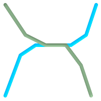
Spatial relationships indicate how two geometries interact with one another. They are a fundamental capability for querying geometry.
According to the OpenGIS Simple Features Implementation Specification for SQL , "the basic approach to comparing two geometries is to make pair-wise tests of the intersections between the Interiors, Boundaries and Exteriors of the two geometries and to classify the relationship between the two geometries based on the entries in the resulting 'intersection' matrix."
In the theory of point-set topology, the points in a geometry embedded in 2-dimensional space are categorized into three sets:
- Boundary
-
The boundary of a geometry is the set of geometries of the next lower dimension. For
POINTs, which have a dimension of 0, the boundary is the empty set. The boundary of aLINESTRINGis the two endpoints. ForPOLYGONs, the boundary is the linework of the exterior and interior rings. - Interior
-
The interior of a geometry are those points of a geometry that are not in the boundary. For
POINTs, the interior is the point itself. The interior of aLINESTRINGis the set of points between the endpoints. ForPOLYGONs, the interior is the areal surface inside the polygon. - Exterior
-
The exterior of a geometry is the rest of the space in which the geometry is embedded; in other words, all points not in the interior or on the boundary of the geometry. It is a 2-dimensional non-closed surface.
The Dimensionally Extended 9-Intersection Model (DE-9IM) describes the spatial relationship between two geometries by specifying the dimensions of the 9 intersections between the above sets for each geometry. The intersection dimensions can be formally represented in a 3x3 intersection matrix .
For a geometry
g
the
Interior
,
Boundary
, and
Exterior
are denoted using the notation
I(g)
,
B(g)
, and
E(g)
.
Also,
dim(s)
denotes the dimension of
a set
s
with the domain of
{0,1,2,F}
:
-
0=> point -
1=> line -
2=> area -
F=> empty set
Using this notation, the intersection matrix for two geometries a and b is:
| Interior | Boundary | Exterior | |
|---|---|---|---|
| Interior | dim( I(a) ∩ I(b) ) | dim( I(a) ∩ B(b) ) | dim( I(a) ∩ E(b) ) |
| Boundary | dim( B(a) ∩ I(b) ) | dim( B(a) ∩ B(b) ) | dim( B(a) ∩ E(b) ) |
| Exterior | dim( E(a) ∩ I(b) ) | dim( E(a) ∩ B(b) ) | dim( E(a) ∩ E(b) ) |
Visually, for two overlapping polygonal geometries, this looks like:
|
||||||||||||||||||
|
|


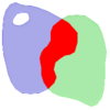

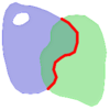
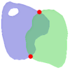
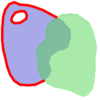

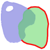

Reading from left to right and top to bottom, the intersection matrix is represented as the text string ' 212101212 '.
For more information, refer to:
To make it easy to determine common spatial relationships, the OGC SFS defines a set of named spatial relationship predicates . PostGIS provides these as the functions ST_Contains , ST_Crosses , ST_Disjoint , ST_Equals , ST_Intersects , ST_Overlaps , ST_Touches , ST_Within . It also defines the non-standard relationship predicates ST_Covers , ST_CoveredBy , and ST_ContainsProperly .
Spatial predicates are usually used as conditions in SQL
WHERE
or
JOIN
clauses.
The named spatial predicates automatically use a spatial index if one is available,
so there is no need to use the bounding box operator
&&
as well.
For example:
SELECT city.name, state.name, city.geom
FROM city JOIN state ON ST_Intersects(city.geom, state.geom);
For more details and illustrations, see the PostGIS Workshop.
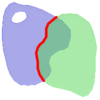
In some cases the named spatial relationships are insufficient to provide a desired spatial filter condition.
For example, consider a linear
dataset representing a road network. It may be required
to identify all road segments that cross
each other, not at a point, but in a line (perhaps to validate some business rule).
In this case
ST_Crosses
does not
provide the necessary spatial filter, since for
linear features it returns
A two-step solution
would be to first compute the actual intersection
(
ST_Intersection
) of pairs of road lines that spatially
intersect (
ST_Intersects
), and then check if the intersection's
ST_GeometryType
is '
Clearly, a simpler and faster solution is desirable. |
|
A second example is locating wharves that intersect a lake's boundary on a line and where one end of the wharf is up on shore. In other words, where a wharf is within but not completely contained by a lake, intersects the boundary of a lake on a line, and where exactly one of the wharf's endpoints is within or on the boundary of the lake. It is possible to use a combination of spatial predicates to find the required features:
|
These requirements can be met by computing the full DE-9IM intersection matrix. PostGIS provides the ST_Relate function to do this:
SELECT ST_Relate( 'LINESTRING (1 1, 5 5)',
                  'POLYGON ((3 3, 3 7, 7 7, 7 3, 3 3))' );
st_relate
-----------
1010F0212
To test a particular spatial relationship,
an
intersection matrix pattern
is used.
This is the matrix representation augmented with the additional symbols
{T,*}
:
-
T=> intersection dimension is non-empty; i.e. is in{0,1,2} -
*=> don't care
Using intersection matrix patterns, specific spatial relationships can be evaluated in a more succinct way. The ST_Relate and the ST_RelateMatch functions can be used to test intersection matrix patterns. For the first example above, the intersection matrix pattern specifying two lines intersecting in a line is ' 1*1***1** ':
-- Find road segments that intersect in a line
SELECT a.id
FROM roads a, roads b
WHERE a.id != b.id
      AND a.geom && b.geom
      AND ST_Relate(a.geom, b.geom, '1*1***1**');
For the second example, the intersection matrix pattern specifying a line partly inside and partly outside a polygon is ' 102101FF2 ':
-- Find wharves partly on a lake's shoreline
SELECT a.lake_id, b.wharf_id
FROM lakes a, wharfs b
WHERE a.geom && b.geom
      AND ST_Relate(a.geom, b.geom, '102101FF2');
When constructing queries using spatial conditions it is important to
ensure that a spatial index is used, if one exists (see
Section 4.1.7, “Building Spatial Indexes”
).
To do this, an index-aware spatial operator or function must be used
in the
WHERE
or
ON
clause.
Spatial operators include
the bounding box-based operators
(of which the most commonly used is
&&
)
and the distance operators used in nearest-neighbour queries
(the most common being
<->
.)
Index-aware functions include most of the named spatial predicates
(such as
ST_Intersects
), and most of the distance predicates
(such as
ST_DWithin
.)
Functions such as ST_Distance do not use indexes to optimize their operation. For example, the following query would be quite slow on a large table:
SELECT the_geom
FROM geom_table
WHERE ST_Distance(the_geom, 'SRID=312;POINT(100000 200000)') < 100
This query selects all the geometries in
geom_table
which are
within 100 units of the point (100000, 200000). It will be slow because
it is calculating the distance between each point in the table and the
specified point, ie. one
ST_Distance()
calculation
is computed for
every
row in the table.
We can reduce the number of rows processed by using the index-aware function ST_DWithin :
SELECT the_geom
FROM geom_table
WHERE ST_DWithin(the_geom, 'SRID=312;POINT(100000 200000)', 100)
This query selects the same geometries, but it does it in a more
efficient way.
This is enabled by
ST_DWithin()
using the
&&
operator internally on an expanded bounding box
of the query geometry.
If there is a spatial index on
the_geom
, the query
planner will recognize that it can use the index to reduce the number of
rows scanned before calculating the distance.
The spatial index allows retrieving only records with geometries
whose bounding boxes overlap the expanded extent
and hence which
might
be within the required distance.
The actual distance is then computed to confirm whether to include the record in the result set.
The examples in this section will make use of two tables, a table
of linear roads, and a table of polygonal municipality boundaries. The
table definitions for the
bc_roads
table is:
Column      | Type              | Description
------------+-------------------+-------------------
gid         | integer           | Unique ID
name        | character varying | Road Name
the_geom    | geometry          | Location Geometry (Linestring)
The table definition for the
bc_municipality
table is:
Column     | Type              | Description
-----------+-------------------+-------------------
gid        | integer           | Unique ID
code       | integer           | Unique ID
name       | character varying | City / Town Name
the_geom   | geometry          | Location Geometry (Polygon)
- 4.2.3.1. What is the total length of all roads, expressed in kilometers?
- 4.2.3.2. How large is the city of Prince George, in hectares?
- 4.2.3.3. What is the largest municipality in the province, by area?
- 4.2.3.4. What is the length of roads fully contained within each municipality?
- 4.2.3.5. Create a new table with all the roads within the city of Prince George.
- 4.2.3.6. What is the length in kilometers of "Douglas St" in Victoria?
- 4.2.3.7. What is the largest municipality polygon that has a hole?
Current PostgreSQL versions (including 9.6) suffer from a query optimizer weakness regarding TOAST tables. TOAST tables are a kind of "extension room" used to store large (in the sense of data size) values that do not fit into normal data pages (like long texts, images or complex geometries with lots of vertices), see the PostgreSQL Documentation for TOAST for more information).
The problem appears if you happen to have a table with rather large geometries, but not too many rows of them (like a table containing the boundaries of all European countries in high resolution). Then the table itself is small, but it uses lots of TOAST space. In our example case, the table itself had about 80 rows and used only 3 data pages, but the TOAST table used 8225 pages.
Now issue a query where you use the geometry operator && to search for a bounding box that matches only very few of those rows. Now the query optimizer sees that the table has only 3 pages and 80 rows. It estimates that a sequential scan on such a small table is much faster than using an index. And so it decides to ignore the GIST index. Usually, this estimation is correct. But in our case, the && operator has to fetch every geometry from disk to compare the bounding boxes, thus reading all TOAST pages, too.
To see whether your suffer from this issue, use the "EXPLAIN ANALYZE" postgresql command. For more information and the technical details, you can read the thread on the postgres performance mailing list: http://archives.postgresql.org/pgsql-performance/2005-02/msg00030.php
and newer thread on PostGIS https://lists.osgeo.org/pipermail/postgis-devel/2017-June/026209.html
The PostgreSQL people are trying to solve this issue by making the query estimation TOAST-aware. For now, here are two workarounds:
The first workaround is to force the query planner to use the index. Send "SET enable_seqscan TO off;" to the server before issuing the query. This basically forces the query planner to avoid sequential scans whenever possible. So it uses the GIST index as usual. But this flag has to be set on every connection, and it causes the query planner to make misestimations in other cases, so you should "SET enable_seqscan TO on;" after the query.
The second workaround is to make the sequential scan as fast as the query planner thinks. This can be achieved by creating an additional column that "caches" the bbox, and matching against this. In our example, the commands are like:
SELECT AddGeometryColumn('myschema','mytable','bbox','4326','GEOMETRY','2');
UPDATE mytable SET bbox = ST_Envelope(ST_Force2D(the_geom));
Now change your query to use the && operator against bbox instead of geom_column, like:
SELECT geom_column
FROM mytable
WHERE bbox && ST_SetSRID('BOX3D(0 0,1 1)'::box3d,4326);
Of course, if you change or add rows to mytable, you have to keep the bbox "in sync". The most transparent way to do this would be triggers, but you also can modify your application to keep the bbox column current or run the UPDATE query above after every modification.
For tables that are mostly read-only, and where a single index is used for the majority of queries, PostgreSQL offers the CLUSTER command. This command physically reorders all the data rows in the same order as the index criteria, yielding two performance advantages: First, for index range scans, the number of seeks on the data table is drastically reduced. Second, if your working set concentrates to some small intervals on the indices, you have a more efficient caching because the data rows are spread along fewer data pages. (Feel invited to read the CLUSTER command documentation from the PostgreSQL manual at this point.)
However, currently PostgreSQL does not allow clustering on PostGIS GIST indices because GIST indices simply ignores NULL values, you get an error message like:
lwgeom=# CLUSTER my_geom_index ON my_table;
ERROR: cannot cluster when index access method does not handle null values
HINT: You may be able to work around this by marking column "the_geom" NOT NULL.
As the HINT message tells you, one can work around this deficiency by adding a "not null" constraint to the table:
lwgeom=# ALTER TABLE my_table ALTER COLUMN the_geom SET not null;
ALTER TABLE
Of course, this will not work if you in fact need NULL values in your geometry column. Additionally, you must use the above method to add the constraint, using a CHECK constraint like "ALTER TABLE blubb ADD CHECK (geometry is not null);" will not work.
Sometimes, you happen to have 3D or 4D data in your table, but always access it using OpenGIS compliant ST_AsText() or ST_AsBinary() functions that only output 2D geometries. They do this by internally calling the ST_Force2D() function, which introduces a significant overhead for large geometries. To avoid this overhead, it may be feasible to pre-drop those additional dimensions once and forever:
UPDATE mytable SET the_geom = ST_Force2D(the_geom);
VACUUM FULL ANALYZE mytable;
Note that if you added your geometry column using AddGeometryColumn() there'll be a constraint on geometry dimension. To bypass it you will need to drop the constraint. Remember to update the entry in the geometry_columns table and recreate the constraint afterwards.
In case of large tables, it may be wise to divide this UPDATE into smaller portions by constraining the UPDATE to a part of the table via a WHERE clause and your primary key or another feasible criteria, and running a simple "VACUUM;" between your UPDATEs. This drastically reduces the need for temporary disk space. Additionally, if you have mixed dimension geometries, restricting the UPDATE by "WHERE dimension(the_geom)>2" skips re-writing of geometries that already are in 2D.
The Minnesota MapServer is an internet web-mapping server which conforms to the OpenGIS Web Map Service specification.
-
The MapServer homepage is at http://mapserver.org .
-
The OpenGIS Web Map Service specification is at http://www.opengeospatial.org/standards/wms .
To use PostGIS with MapServer, you need to know how to configure MapServer, which is beyond the scope of this documentation. This section covers specific PostGIS issues and configuration details.
To use PostGIS with MapServer, you will need:
-
Version 0.6 or newer of PostGIS.
-
Version 3.5 or newer of MapServer.
MapServer accesses PostGIS/PostgreSQL data like any other
PostgreSQL client, using the
libpq
interface. This means that
MapServer can be installed on any machine with network access to the
PostGIS server, and use PostGIS as a source of data. The faster the connection
between the systems, the better.
-
Compile and install MapServer, with whatever options you desire, including the "--with-postgis" configuration option.
-
In your MapServer map file, add a PostGIS layer. For example:
LAYER
  CONNECTIONTYPE postgis
  NAME "widehighways"
  # Connect to a remote spatial database
  CONNECTION "user=dbuser dbname=gisdatabase host=bigserver"
  PROCESSING "CLOSE_CONNECTION=DEFER"
  # Get the lines from the 'geom' column of the 'roads' table
  DATA "geom from roads using srid=4326 using unique gid"
  STATUS ON
  TYPE LINE
  # Of the lines in the extents, only render the wide highways
  FILTER "type = 'highway' and numlanes >= 4"
  CLASS
    # Make the superhighways brighter and 2 pixels wide
    EXPRESSION ([numlanes] >= 6)
    STYLE
      COLOR 255 22 22
      WIDTH 2
    END
  END
  CLASS
    # All the rest are darker and only 1 pixel wide
    EXPRESSION ([numlanes] < 6)
    STYLE
      COLOR 205 92 82
    END
  END
END
In the example above, the PostGIS-specific directives are as follows:
- CONNECTIONTYPE
-
For PostGIS layers, this is always "postgis".
- CONNECTION
-
The database connection is governed by the a 'connection string' which is a standard set of keys and values like this (with the default values in <>):
user=<username> password=<password> dbname=<username> hostname=<server> port=<5432>
An empty connection string is still valid, and any of the key/value pairs can be omitted. At a minimum you will generally supply the database name and username to connect with.
- DATA
-
The form of this parameter is "<geocolumn> from <tablename> using srid=<srid> using unique <primary key>" where the column is the spatial column to be rendered to the map, the SRID is SRID used by the column and the primary key is the table primary key (or any other uniquely-valued column with an index).
You can omit the "using srid" and "using unique" clauses and MapServer will automatically determine the correct values if possible, but at the cost of running a few extra queries on the server for each map draw.
- PROCESSING
-
Putting in a CLOSE_CONNECTION=DEFER if you have multiple layers reuses existing connections instead of closing them. This improves speed. Refer to for MapServer PostGIS Performance Tips for a more detailed explanation.
- FILTER
-
The filter must be a valid SQL string corresponding to the logic normally following the "WHERE" keyword in a SQL query. So, for example, to render only roads with 6 or more lanes, use a filter of "num_lanes >= 6".
-
In your spatial database, ensure you have spatial (GiST) indexes built for any the layers you will be drawing.
CREATE INDEX [indexname] ON [tablename] USING GIST ( [geometrycolumn] );
-
If you will be querying your layers using MapServer you will also need to use the "using unique" clause in your DATA statement.
MapServer requires unique identifiers for each spatial record when doing queries, and the PostGIS module of MapServer uses the unique value you specify in order to provide these unique identifiers. Using the table primary key is the best practice.
- 4.4.1.2.1. When I use an EXPRESSION in my map file, the condition never returns as true, even though I know the values exist in my table.
- 4.4.1.2.2. The FILTER I use for my Shapefiles is not working for my PostGIS table of the same data.
- 4.4.1.2.3. My PostGIS layer draws much slower than my Shapefile layer, is this normal?
- 4.4.1.2.4. My PostGIS layer draws fine, but queries are really slow. What is wrong?
- 4.4.1.2.5. Can I use "geography" columns (new in PostGIS 1.5) as a source for MapServer layers?
The
USING
pseudo-SQL clause is used to add some
information to help mapserver understand the results of more complex
queries. More specifically, when either a view or a subselect is used as
the source table (the thing to the right of "FROM" in a
DATA
definition) it is more difficult for mapserver
to automatically determine a unique identifier for each row and also the
SRID for the table. The
USING
clause can provide
mapserver with these two pieces of information as follows:
DATA "geom FROM (
  SELECT
    table1.geom AS geom,
    table1.gid AS gid,
    table2.data AS data
  FROM table1
  LEFT JOIN table2
  ON table1.id = table2.id
) AS new_table USING UNIQUE gid USING SRID=4326"
- USING UNIQUE <uniqueid>
-
MapServer requires a unique id for each row in order to identify the row when doing map queries. Normally it identifies the primary key from the system tables. However, views and subselects don't automatically have an known unique column. If you want to use MapServer's query functionality, you need to ensure your view or subselect includes a uniquely valued column, and declare it with
USING UNIQUE. For example, you could explicitly select nee of the table's primary key values for this purpose, or any other column which is guaranteed to be unique for the result set.
"Querying a Map" is the action of clicking on a map to ask for information about the map features in that location. Don't confuse "map queries" with the SQL query in a
DATAdefinition. - USING SRID=<srid>
-
PostGIS needs to know which spatial referencing system is being used by the geometries in order to return the correct data back to MapServer. Normally it is possible to find this information in the "geometry_columns" table in the PostGIS database, however, this is not possible for tables which are created on the fly such as subselects and views. So the
USING SRID=option allows the correct SRID to be specified in theDATAdefinition.
Lets start with a simple example and work our way up. Consider the following MapServer layer definition:
LAYER
  CONNECTIONTYPE postgis
  NAME "roads"
  CONNECTION "user=theuser password=thepass dbname=thedb host=theserver"
  DATA "geom from roads"
  STATUS ON
  TYPE LINE
  CLASS
    STYLE
      COLOR 0 0 0
    END
  END
END
This layer will display all the road geometries in the roads table as black lines.
Now lets say we want to show only the highways until we get zoomed in to at least a 1:100000 scale - the next two layers will achieve this effect:
LAYER
  CONNECTIONTYPE postgis
  CONNECTION "user=theuser password=thepass dbname=thedb host=theserver"
  PROCESSING "CLOSE_CONNECTION=DEFER"
  DATA "geom from roads"
  MINSCALE 100000
  STATUS ON
  TYPE LINE
  FILTER "road_type = 'highway'"
  CLASS
    COLOR 0 0 0
  END
END
LAYER
  CONNECTIONTYPE postgis
  CONNECTION "user=theuser password=thepass dbname=thedb host=theserver"
  PROCESSING "CLOSE_CONNECTION=DEFER"
  DATA "geom from roads"
  MAXSCALE 100000
  STATUS ON
  TYPE LINE
  CLASSITEM road_type
  CLASS
    EXPRESSION "highway"
    STYLE
      WIDTH 2
      COLOR 255 0 0
    END
  END
  CLASS
    STYLE
      COLOR 0 0 0
    END
  END
END
The first layer is used when the scale is greater than 1:100000,
and displays only the roads of type "highway" as black lines. The
FILTER
option causes only roads of type "highway" to
be displayed.
The second layer is used when the scale is less than 1:100000, and will display highways as double-thick red lines, and other roads as regular black lines.
So, we have done a couple of interesting things using only
MapServer functionality, but our
DATA
SQL statement
has remained simple. Suppose that the name of the road is stored in
another table (for whatever reason) and we need to do a join to get it
and label our roads.
LAYER
  CONNECTIONTYPE postgis
  CONNECTION "user=theuser password=thepass dbname=thedb host=theserver"
  DATA "geom FROM (SELECT roads.gid AS gid, roads.geom AS geom,
        road_names.name as name FROM roads LEFT JOIN road_names ON
        roads.road_name_id = road_names.road_name_id)
        AS named_roads USING UNIQUE gid USING SRID=4326"
  MAXSCALE 20000
  STATUS ON
  TYPE ANNOTATION
  LABELITEM name
  CLASS
    LABEL
      ANGLE auto
      SIZE 8
      COLOR 0 192 0
      TYPE truetype
      FONT arial
    END
  END
END
This annotation layer adds green labels to all the roads when the
scale gets down to 1:20000 or less. It also demonstrates how to use an
SQL join in a
DATA
definition.
Java clients can access PostGIS "geometry" objects in the PostgreSQL database either directly as text representations or using the JDBC extension objects bundled with PostGIS. In order to use the extension objects, the "postgis.jar" file must be in your CLASSPATH along with the "postgresql.jar" JDBC driver package.
import java.sql.*;
import java.util.*;
import java.lang.*;
import org.postgis.*;

public class JavaGIS {

public static void main(String[] args) {

  java.sql.Connection conn;

  try {
    /*
    * Load the JDBC driver and establish a connection.
    */
    Class.forName("org.postgresql.Driver");
    String url = "jdbc:postgresql://localhost:5432/database";
    conn = DriverManager.getConnection(url, "postgres", "");
    /*
    * Add the geometry types to the connection. Note that you
    * must cast the connection to the pgsql-specific connection
    * implementation before calling the addDataType() method.
    */
    ((org.postgresql.PGConnection)conn).addDataType("geometry",Class.forName("org.postgis.PGgeometry"));
    ((org.postgresql.PGConnection)conn).addDataType("box3d",Class.forName("org.postgis.PGbox3d"));
    /*
    * Create a statement and execute a select query.
    */
    Statement s = conn.createStatement();
    ResultSet r = s.executeQuery("select geom,id from geomtable");
    while( r.next() ) {
      /*
      * Retrieve the geometry as an object then cast it to the geometry type.
      * Print things out.
      */
      PGgeometry geom = (PGgeometry)r.getObject(1);
      int id = r.getInt(2);
      System.out.println("Row " + id + ":");
      System.out.println(geom.toString());
    }
    s.close();
    conn.close();
  }
catch( Exception e ) {
  e.printStackTrace();
  }
}
}
The "PGgeometry" object is a wrapper object which contains a specific topological geometry object (subclasses of the abstract class "Geometry") depending on the type: Point, LineString, Polygon, MultiPoint, MultiLineString, MultiPolygon.
PGgeometry geom = (PGgeometry)r.getObject(1);
if( geom.getType() == Geometry.POLYGON ) {
  Polygon pl = (Polygon)geom.getGeometry();
  for( int r = 0; r < pl.numRings(); r++) {
    LinearRing rng = pl.getRing(r);
    System.out.println("Ring: " + r);
    for( int p = 0; p < rng.numPoints(); p++ ) {
      Point pt = rng.getPoint(p);
      System.out.println("Point: " + p);
      System.out.println(pt.toString());
    }
  }
}
The JavaDoc for the extension objects provides a reference for the various data accessor functions in the geometric objects.
...
For most use cases, you will create PostGIS rasters by loading existing raster files using the packaged
raster2pgsql
raster loader.
The
raster2pgsql
is a raster loader executable that loads GDAL supported raster formats into sql suitable for loading into a PostGIS raster table.
It is capable of loading folders of raster files as well as creating overviews of rasters.
Since the raster2pgsql is compiled as part of PostGIS most often (unless you compile your own GDAL library), the raster types supported
by the executable will be the same as those compiled in the GDAL dependency library. To get a list of raster types your particular raster2pgsql supports use the
-G
switch. These should be the same as those provided by your PostGIS install documented here
ST_GDALDrivers
if you are using the same gdal library for both.
|
|
|
|
The older version of this tool was a python script. The executable has replaced the python script. If you still find the need for the Python script Examples of the python one can be found at GDAL PostGIS Raster Driver Usage . Please note that the raster2pgsql python script may not work with future versions of PostGIS raster and is no longer supported. |
|
|
|
|
When creating overviews of a specific factor from a set of rasters that are aligned, it is possible for the overviews to not align. Visit http://trac.osgeo.org/postgis/ticket/1764 for an example where the overviews do not align. |
EXAMPLE USAGE:
raster2pgsqlraster_options_go_hereraster_filesomeschema.sometable> out.sql
- -?
-
Display help screen. Help will also display if you don't pass in any arguments.
- -G
-
Print the supported raster formats.
- (c|a|d|p) These are mutually exclusive options:
-
- -c
-
Create new table and populate it with raster(s), this is the default mode
- -a
-
Append raster(s) to an existing table.
- -d
-
Drop table, create new one and populate it with raster(s)
- -p
-
Prepare mode, only create the table.
- Raster processing: Applying constraints for proper registering in raster catalogs
-
- -C
-
Apply raster constraints -- srid, pixelsize etc. to ensure raster is properly registered in
raster_columnsview. - -x
-
Disable setting the max extent constraint. Only applied if -C flag is also used.
- -r
-
Set the constraints (spatially unique and coverage tile) for regular blocking. Only applied if -C flag is also used.
- Raster processing: Optional parameters used to manipulate input raster dataset
-
- -s <SRID>
-
Assign output raster with specified SRID. If not provided or is zero, raster's metadata will be checked to determine an appropriate SRID.
- -b BAND
-
Index (1-based) of band to extract from raster. For more than one band index, separate with comma (,). If unspecified, all bands of raster will be extracted.
- -t TILE_SIZE
-
Cut raster into tiles to be inserted one per table row.
TILE_SIZEis expressed as WIDTHxHEIGHT or set to the value "auto" to allow the loader to compute an appropriate tile size using the first raster and applied to all rasters. - -P
-
Pad right-most and bottom-most tiles to guarantee that all tiles have the same width and height.
- -R, --register
-
Register the raster as a filesystem (out-db) raster.
Only the metadata of the raster and path location to the raster is stored in the database (not the pixels).
-
-l
OVERVIEW_FACTOR -
Create overview of the raster. For more than one factor, separate with comma(,). Overview table name follows the pattern o_
overview factor_table, whereoverview factoris a placeholder for numerical overview factor andtableis replaced with the base table name. Created overview is stored in the database and is not affected by -R. Note that your generated sql file will contain both the main table and overview tables. -
-N
NODATA -
NODATA value to use on bands without a NODATA value.
- Optional parameters used to manipulate database objects
-
- -f COLUMN
-
Specify name of destination raster column, default is 'rast'
- -F
-
Add a column with the name of the file
- -n COLUMN
-
Specify the name of the filename column. Implies -F.
- -q
-
Wrap PostgreSQL identifiers in quotes.
- -I
-
Create a GiST index on the raster column.
- -M
-
Vacuum analyze the raster table.
- -k
-
Skip NODATA value checks for each raster band.
-
-T
tablespace -
Specify the tablespace for the new table. Note that indices (including the primary key) will still use the default tablespace unless the -X flag is also used.
-
-X
tablespace -
Specify the tablespace for the table's new index. This applies to the primary key and the spatial index if the -I flag is used.
- -Y
-
Use copy statements instead of insert statements.
- -e
-
Execute each statement individually, do not use a transaction.
- -E ENDIAN
-
Control endianness of generated binary output of raster; specify 0 for XDR and 1 for NDR (default); only NDR output is supported now
-
-V
version -
Specify version of output format. Default is 0. Only 0 is supported at this time.
An example session using the loader to create an input file and uploading it chunked in 100x100 tiles might look like this:
|
|
|
|
You can leave the schema name out e.g
|
raster2pgsql -s 4326 -I -C -M *.tif -F -t 100x100 public.demelevation > elev.sql
psql -d gisdb -f elev.sql
A conversion and upload can be done all in one step using UNIX pipes:
raster2pgsql -s 4326 -I -C -M *.tif -F -t 100x100 public.demelevation | psql -d gisdb
Load rasters Massachusetts state plane meters aerial tiles
into a schema called
aerial
and create a full view, 2 and 4 level overview tables, use copy mode for inserting (no intermediary file just straight to db), and -e don't force everything in a transaction (good if you want to see data in tables right away without waiting). Break up the rasters into 128x128 pixel tiles and apply raster constraints. Use copy mode instead of table insert. (-F) Include a field called filename to hold the name of the file the tiles were cut from.
raster2pgsql -I -C -e -Y -F -s 26986 -t 128x128 -l 2,4 bostonaerials2008/*.jpg aerials.boston | psql -U postgres -d gisdb -h localhost -p 5432
--get a list of raster types supported:
raster2pgsql -G
The -G commands outputs a list something like
Available GDAL raster formats:
  Virtual Raster
  GeoTIFF
  National Imagery Transmission Format
  Raster Product Format TOC format
  ECRG TOC format
  Erdas Imagine Images (.img)
  CEOS SAR Image
  CEOS Image
  JAXA PALSAR Product Reader (Level 1.1/1.5)
  Ground-based SAR Applications Testbed File Format (.gff)
  ELAS
  Arc/Info Binary Grid
  Arc/Info ASCII Grid
  GRASS ASCII Grid
  SDTS Raster
  DTED Elevation Raster
  Portable Network Graphics
  JPEG JFIF
  In Memory Raster
  Japanese DEM (.mem)
  Graphics Interchange Format (.gif)
  Graphics Interchange Format (.gif)
  Envisat Image Format
  Maptech BSB Nautical Charts
  X11 PixMap Format
  MS Windows Device Independent Bitmap
  SPOT DIMAP
  AirSAR Polarimetric Image
  RadarSat 2 XML Product
  PCIDSK Database File
  PCRaster Raster File
  ILWIS Raster Map
  SGI Image File Format 1.0
  SRTMHGT File Format
  Leveller heightfield
  Terragen heightfield
  USGS Astrogeology ISIS cube (Version 3)
  USGS Astrogeology ISIS cube (Version 2)
  NASA Planetary Data System
  EarthWatch .TIL
  ERMapper .ers Labelled
  NOAA Polar Orbiter Level 1b Data Set
  FIT Image
  GRIdded Binary (.grb)
  Raster Matrix Format
  EUMETSAT Archive native (.nat)
  Idrisi Raster A.1
  Intergraph Raster
  Golden Software ASCII Grid (.grd)
  Golden Software Binary Grid (.grd)
  Golden Software 7 Binary Grid (.grd)
  COSAR Annotated Binary Matrix (TerraSAR-X)
  TerraSAR-X Product
  DRDC COASP SAR Processor Raster
  R Object Data Store
  Portable Pixmap Format (netpbm)
  USGS DOQ (Old Style)
  USGS DOQ (New Style)
  ENVI .hdr Labelled
  ESRI .hdr Labelled
  Generic Binary (.hdr Labelled)
  PCI .aux Labelled
  Vexcel MFF Raster
  Vexcel MFF2 (HKV) Raster
  Fuji BAS Scanner Image
  GSC Geogrid
  EOSAT FAST Format
  VTP .bt (Binary Terrain) 1.3 Format
  Erdas .LAN/.GIS
  Convair PolGASP
  Image Data and Analysis
  NLAPS Data Format
  Erdas Imagine Raw
  DIPEx
  FARSITE v.4 Landscape File (.lcp)
  NOAA Vertical Datum .GTX
  NADCON .los/.las Datum Grid Shift
  NTv2 Datum Grid Shift
  ACE2
  Snow Data Assimilation System
  Swedish Grid RIK (.rik)
  USGS Optional ASCII DEM (and CDED)
  GeoSoft Grid Exchange Format
  Northwood Numeric Grid Format .grd/.tab
  Northwood Classified Grid Format .grc/.tab
  ARC Digitized Raster Graphics
  Standard Raster Product (ASRP/USRP)
  Magellan topo (.blx)
  SAGA GIS Binary Grid (.sdat)
  Kml Super Overlay
  ASCII Gridded XYZ
  HF2/HFZ heightfield raster
  OziExplorer Image File
  USGS LULC Composite Theme Grid
  Arc/Info Export E00 GRID
  ZMap Plus Grid
  NOAA NGS Geoid Height Grids
On many occasions, you'll want to create rasters and raster tables right in the database. There are a plethora of functions to do that. The general steps to follow.
-
Create a table with a raster column to hold the new raster records which can be accomplished with:
CREATE TABLE myrasters(rid serial primary key, rast raster);
-
There are many functions to help with that goal. If you are creating rasters not as a derivative of other rasters, you will want to start with: ST_MakeEmptyRaster , followed by ST_AddBand
You can also create rasters from geometries. To achieve that you'll want to use ST_AsRaster perhaps accompanied with other functions such as ST_Union or ST_MapAlgebraFct or any of the family of other map algebra functions.
There are even many more options for creating new raster tables from existing tables. For example you can create a raster table in a different projection from an existing one using ST_Transform
-
Once you are done populating your table initially, you'll want to create a spatial index on the raster column with something like:
CREATE INDEX myrasters_rast_st_convexhull_idx ON myrasters USING gist( ST_ConvexHull(rast) );
Note the use of ST_ConvexHull since most raster operators are based on the convex hull of the rasters.
Pre-2.0 versions of PostGIS raster were based on the envelop rather than the convex hull. For the spatial indexes to work properly you'll need to drop those and replace with convex hull based index.
-
Apply raster constraints using AddRasterConstraints
There are two raster catalog views that come packaged with PostGIS. Both views utilize information embedded in the constraints of the raster tables. As a result the catalog views are always consistent with the raster data in the tables since the constraints are enforced.
-
raster_columnsthis view catalogs all the raster table columns in your database. -
raster_overviewsthis view catalogs all the raster table columns in your database that serve as overviews for a finer grained table. Tables of this type are generated when you use the-lswitch during load.
The
raster_columns
is a catalog of all raster table columns in your database that are of type raster. It is a view utilizing the constraints on the tables
so the information is always consistent even if you restore one raster table from a backup of another database. The following columns exist in the
raster_columns
catalog.
If you created your tables not with the loader or forgot to specify the
-C
flag during load, you can enforce the constraints after the
fact using
AddRasterConstraints
so that the
raster_columns
catalog registers the common information about your raster tiles.
-
r_table_catalogThe database the table is in. This will always read the current database. -
r_table_schemaThe database schema the raster table belongs to. -
r_table_nameraster table -
r_raster_columnthe column in ther_table_nametable that is of type raster. There is nothing in PostGIS preventing you from having multiple raster columns per table so its possible to have a raster table listed multiple times with a different raster column for each. -
sridThe spatial reference identifier of the raster. Should be an entry in the Section 4.1.3.1, “The SPATIAL_REF_SYS Table and Spatial Reference Systems” . -
scale_xThe scaling between geometric spatial coordinates and pixel. This is only available if all tiles in the raster column have the samescale_xand this constraint is applied. Refer to ST_ScaleX for more details. -
scale_yThe scaling between geometric spatial coordinates and pixel. This is only available if all tiles in the raster column have the samescale_yand thescale_yconstraint is applied. Refer to ST_ScaleY for more details. -
blocksize_xThe width (number of pixels across) of each raster tile . Refer to ST_Width for more details. -
blocksize_yThe width (number of pixels down) of each raster tile . Refer to ST_Height for more details. -
same_alignmentA boolean that is true if all the raster tiles have the same alignment . Refer to ST_SameAlignment for more details. -
regular_blockingIf the raster column has the spatially unique and coverage tile constraints, the value with be TRUE. Otherwise, it will be FALSE. -
num_bandsThe number of bands in each tile of your raster set. This is the same information as what is provided by ST_NumBands -
pixel_typesAn array defining the pixel type for each band. You will have the same number of elements in this array as you have number of bands. The pixel_types are one of the following defined in ST_BandPixelType . -
nodata_valuesAn array of double precision numbers denoting thenodata_valuefor each band. You will have the same number of elements in this array as you have number of bands. These numbers define the pixel value for each band that should be ignored for most operations. This is similar information provided by ST_BandNoDataValue . -
out_dbAn array of boolean flags indicating if the raster bands data is maintained outside the database. You will have the same number of elements in this array as you have number of bands. -
extentThis is the extent of all the raster rows in your raster set. If you plan to load more data that will change the extent of the set, you'll want to run the DropRasterConstraints function before load and then reapply constraints with AddRasterConstraints after load. -
spatial_indexA boolean that is true if raster column has a spatial index.
raster_overviews
catalogs information about raster table columns used for overviews and additional information about them that is useful to know when utilizing overviews. Overview tables are cataloged in both
raster_columns
and
raster_overviews
because they are rasters in their own right but also serve an additional special purpose of being a lower resolution caricature of a higher resolution table. These are generated along-side the main raster table when you use the
-l
switch in raster loading or can be generated manually using
AddOverviewConstraints
.
Overview tables contain the same constraints as other raster tables as well as additional informational only constraints specific to overviews.
|
|
|
|
The information in
|
Two main reasons for overviews are:
-
Low resolution representation of the core tables commonly used for fast mapping zoom-out.
-
Computations are generally faster to do on them than their higher resolution parents because there are fewer records and each pixel covers more territory. Though the computations are not as accurate as the high-res tables they support, they can be sufficient in many rule-of-thumb computations.
The
raster_overviews
catalog contains the following columns of information.
-
o_table_catalogThe database the overview table is in. This will always read the current database. -
o_table_schemaThe database schema the overview raster table belongs to. -
o_table_nameraster overview table name -
o_raster_columnthe raster column in the overview table. -
r_table_catalogThe database the raster table that this overview services is in. This will always read the current database. -
r_table_schemaThe database schema the raster table that this overview services belongs to. -
r_table_nameraster table that this overview services. -
r_raster_columnthe raster column that this overview column services. -
overview_factor- this is the pyramid level of the overview table. The higher the number the lower the resolution of the table. raster2pgsql if given a folder of images, will compute overview of each image file and load separately. Level 1 is assumed and always the original file. Level 2 is will have each tile represent 4 of the original. So for example if you have a folder of 5000x5000 pixel image files that you chose to chunk 125x125, for each image file your base table will have (5000*5000)/(125*125) records = 1600, your (l=2)o_2table will have ceiling(1600/Power(2,2)) = 400 rows, your (l=3)o_3will have ceiling(1600/Power(2,3) ) = 200 rows. If your pixels aren't divisible by the size of your tiles, you'll get some scrap tiles (tiles not completely filled). Note that each overview tile generated by raster2pgsql has the same number of pixels as its parent, but is of a lower resolution where each pixel of it represents (Power(2,overview_factor) pixels of the original).
- 4.5.3.1. PHP Example Outputting using ST_AsPNG in concert with other raster functions
- 4.5.3.2. ASP.NET C# Example Outputting using ST_AsPNG in concert with other raster functions
- 4.5.3.3. Java console app that outputs raster query as Image file
- 4.5.3.4. Use PLPython to dump out images via SQL
- 4.5.3.5. Outputting Rasters with PSQL
The fact that PostGIS raster provides you with SQL functions to render rasters in known image formats gives you a lot of optoins for rendering them. For example you can use OpenOffice / LibreOffice for rendering as demonstrated in Rendering PostGIS Raster graphics with LibreOffice Base Reports . In addition you can use a wide variety of languages as demonstrated in this section.
In this section, we'll demonstrate how to use the PHP PostgreSQL driver and the ST_AsGDALRaster family of functions to output band 1,2,3 of a raster to a PHP request stream that can then be embedded in an img src html tag.
The sample query demonstrates how to combine a whole bunch of raster functions together to grab all tiles that intersect a particular wgs 84 bounding box and then unions with ST_Union the intersecting tiles together returning all bands, transforms to user specified projection using ST_Transform , and then outputs the results as a png using ST_AsPNG .
You would call the below using
http://mywebserver/test_raster.php?srid=2249
to get the raster image in Massachusetts state plane feet.
<?php
/** contents of test_raster.php **/
$conn_str ='dbname=mydb host=localhost port=5432 user=myuser password=mypwd';
$dbconn = pg_connect($conn_str);
header('Content-Type: image/png');
/**If a particular projection was requested use it otherwise use mass state plane meters **/
if (!empty( $_REQUEST['srid'] ) && is_numeric( $_REQUEST['srid']) ){
		$input_srid = intval($_REQUEST['srid']);
}
else { $input_srid = 26986; }
/** The set bytea_output may be needed for PostgreSQL 9.0+, but not for 8.4 **/
$sql = "set bytea_output='escape';
SELECT ST_AsPNG(ST_Transform(
			ST_AddBand(ST_Union(rast,1), ARRAY[ST_Union(rast,2),ST_Union(rast,3)])
				,$input_srid) ) As new_rast
 FROM aerials.boston
	WHERE
	 ST_Intersects(rast, ST_Transform(ST_MakeEnvelope(-71.1217, 42.227, -71.1210, 42.218,4326),26986) )";
$result = pg_query($sql);
$row = pg_fetch_row($result);
pg_free_result($result);
if ($row === false) return;
echo pg_unescape_bytea($row[0]);
?>
In this section, we'll demonstrate how to use Npgsql PostgreSQL .NET driver and the ST_AsGDALRaster family of functions to output band 1,2,3 of a raster to a PHP request stream that can then be embedded in an img src html tag.
You will need the npgsql .NET PostgreSQL driver for this exercise which you can get the latest of from http://npgsql.projects.postgresql.org/ . Just download the latest and drop into your ASP.NET bin folder and you'll be good to go.
The sample query demonstrates how to combine a whole bunch of raster functions together to grab all tiles that intersect a particular wgs 84 bounding box and then unions with ST_Union the intersecting tiles together returning all bands, transforms to user specified projection using ST_Transform , and then outputs the results as a png using ST_AsPNG .
This is same example as Section 4.5.3.1, “PHP Example Outputting using ST_AsPNG in concert with other raster functions” except implemented in C#.
You would call the below using
http://mywebserver/TestRaster.ashx?srid=2249
to get the raster image in Massachusetts state plane feet.
 -- web.config connection string section --
<connectionStrings>
    <add name="DSN"
        connectionString="server=localhost;database=mydb;Port=5432;User Id=myuser;password=mypwd"/>
</connectionStrings>
// Code for TestRaster.ashx
<%@ WebHandler Language="C#" Class="TestRaster" %>
using System;
using System.Data;
using System.Web;
using Npgsql;

public class TestRaster : IHttpHandler
{
	public void ProcessRequest(HttpContext context)
	{

		context.Response.ContentType = "image/png";
		context.Response.BinaryWrite(GetResults(context));

	}

	public bool IsReusable {
		get { return false; }
	}

	public byte[] GetResults(HttpContext context)
	{
		byte[] result = null;
		NpgsqlCommand command;
		string sql = null;
		int input_srid = 26986;
        try {
		    using (NpgsqlConnection conn = new NpgsqlConnection(System.Configuration.ConfigurationManager.ConnectionStrings["DSN"].ConnectionString)) {
			    conn.Open();

                if (context.Request["srid"] != null)
                {
                    input_srid = Convert.ToInt32(context.Request["srid"]);
                }
                sql = @"SELECT ST_AsPNG(
                            ST_Transform(
			                ST_AddBand(
                                ST_Union(rast,1), ARRAY[ST_Union(rast,2),ST_Union(rast,3)])
				                    ,:input_srid) ) As new_rast
                        FROM aerials.boston
	                        WHERE
	                            ST_Intersects(rast,
                                    ST_Transform(ST_MakeEnvelope(-71.1217, 42.227, -71.1210, 42.218,4326),26986) )";
			    command = new NpgsqlCommand(sql, conn);
                command.Parameters.Add(new NpgsqlParameter("input_srid", input_srid));


			    result = (byte[]) command.ExecuteScalar();
                conn.Close();
			}

		}
        catch (Exception ex)
        {
            result = null;
            context.Response.Write(ex.Message.Trim());
        }
		return result;
	}
}
This is a simple java console app that takes a query that returns one image and outputs to specified file.
You can download the latest PostgreSQL JDBC drivers from http://jdbc.postgresql.org/download.html
You can compile the following code using a command something like:
set env CLASSPATH .:..\postgresql-9.0-801.jdbc4.jar
javac SaveQueryImage.java
jar cfm SaveQueryImage.jar Manifest.txt *.class
And call it from the command-line with something like
java -jar SaveQueryImage.jar "SELECT ST_AsPNG(ST_AsRaster(ST_Buffer(ST_Point(1,5),10, 'quad_segs=2'),150, 150, '8BUI',100));" "test.png"
 -- Manifest.txt --
Class-Path: postgresql-9.0-801.jdbc4.jar
Main-Class: SaveQueryImage
// Code for SaveQueryImage.java
import java.sql.Connection;
import java.sql.SQLException;
import java.sql.PreparedStatement;
import java.sql.ResultSet;
import java.io.*;

public class SaveQueryImage {
  public static void main(String[] argv) {
      System.out.println("Checking if Driver is registered with DriverManager.");

      try {
        //java.sql.DriverManager.registerDriver (new org.postgresql.Driver());
        Class.forName("org.postgresql.Driver");
      }
      catch (ClassNotFoundException cnfe) {
        System.out.println("Couldn't find the driver!");
        cnfe.printStackTrace();
        System.exit(1);
      }

      Connection conn = null;

      try {
        conn = DriverManager.getConnection("jdbc:postgresql://localhost:5432/mydb","myuser", "mypwd");
        conn.setAutoCommit(false);

        PreparedStatement sGetImg = conn.prepareStatement(argv[0]);

        ResultSet rs = sGetImg.executeQuery();

		FileOutputStream fout;
		try
		{
			rs.next();
			/** Output to file name requested by user **/
			fout = new FileOutputStream(new File(argv[1]) );
			fout.write(rs.getBytes(1));
			fout.close();
		}
		catch(Exception e)
		{
			System.out.println("Can't create file");
			e.printStackTrace();
		}

        rs.close();
		sGetImg.close();
        conn.close();
      }
      catch (SQLException se) {
        System.out.println("Couldn't connect: print out a stack trace and exit.");
        se.printStackTrace();
        System.exit(1);
      }
  }
}
This is a plpython stored function that creates a file in the server directory for each record. Requires you have plpython installed. Should work fine with both plpythonu and plpython3u.
CREATE OR REPLACE FUNCTION write_file (param_bytes bytea, param_filepath text)
RETURNS text
AS $$
f = open(param_filepath, 'wb+')
f.write(param_bytes)
return param_filepath
$$ LANGUAGE plpythonu;
--write out 5 images to the PostgreSQL server in varying sizes
-- note the postgresql daemon account needs to have write access to folder
-- this echos back the file names created;
 SELECT write_file(ST_AsPNG(
	ST_AsRaster(ST_Buffer(ST_Point(1,5),j*5, 'quad_segs=2'),150*j, 150*j, '8BUI',100)),
	 'C:/temp/slices'|| j || '.png')
	 FROM generate_series(1,5) As j;

     write_file
---------------------
 C:/temp/slices1.png
 C:/temp/slices2.png
 C:/temp/slices3.png
 C:/temp/slices4.png
 C:/temp/slices5.png
Sadly PSQL doesn't have easy to use built-in functionality for outputting binaries. This is a bit of a hack that piggy backs on PostgreSQL somewhat legacy large object support. To use first launch your psql commandline connected to your database.
Unlike the python approach, this approach creates the file on your local computer.
SELECT oid, lowrite(lo_open(oid, 131072), png) As num_bytes
 FROM
 ( VALUES (lo_create(0),
   ST_AsPNG( (SELECT rast FROM aerials.boston WHERE rid=1) )
  ) ) As v(oid,png);
-- you'll get an output something like --
   oid   | num_bytes
---------+-----------
 2630819 |     74860

-- next note the oid and do this replacing the c:/test.png to file path location
-- on your local computer
 \lo_export 2630819 'C:/temp/aerial_samp.png'

-- this deletes the file from large object storage on db
SELECT lo_unlink(2630819);
- 4.6.1. Topology Types
- 4.6.2. Topology Domains
- 4.6.3. Topology and TopoGeometry Management
- 4.6.4. Topology Statistics Management
- 4.6.5. Topology Constructors
- 4.6.6. Topology Editors
- 4.6.7. Topology Accessors
- 4.6.8. Topology Processing
- 4.6.9. TopoGeometry Constructors
- 4.6.10. TopoGeometry Editors
- 4.6.11. TopoGeometry Accessors
- 4.6.12. TopoGeometry Outputs
- 4.6.13. Topology Spatial Relationships
The PostGIS Topology types and functions are used to manage topological objects such as faces, edges and nodes.
Sandro Santilli's presentation at PostGIS Day Paris 2011 conference gives a good synopsis of PostGIS Topology and where it is headed Topology with PostGIS 2.0 slide deck .
Vincent Picavet provides a good synopsis and overview of what is Topology, how is it used, and various FOSS4G tools that support it in PostGIS Topology PGConf EU 2012 .
An example of a topologically based GIS database is the US Census Topologically Integrated Geographic Encoding and Referencing System (TIGER) database. If you want to experiment with PostGIS topology and need some data, check out Topology_Load_Tiger .
The PostGIS topology module has existed in prior versions of PostGIS but was never part of the Official PostGIS documentation. In PostGIS 2.0.0 major cleanup is going on to remove use of all deprecated functions in it, fix known usability issues, better document the features and functions, add new functions, and enhance to closer conform to SQL-MM standards.
Details of this project can be found at PostGIS Topology Wiki
All functions and tables associated with this module are installed in a schema called
topology
.
Functions that are defined in SQL/MM standard are prefixed with ST_ and functions specific to PostGIS are not prefixed.
Topology support is build by default starting with PostGIS 2.0, and can be disabled specifying --without-topology configure option at build time as described in Chapter 2, PostGIS Installation
-
getfaceedges_returntype
— A composite type that consists of a sequence number and edge number. This is the return type for
ST_GetFaceEdges. - TopoGeometry — A composite type representing a topologically defined geometry.
-
validatetopology_returntype
— A composite type that consists of an error message and id1 and id2 to denote location of error. This is the return type for
ValidateTopology.
This section lists the PostgreSQL domains installed by PostGIS Topology. Domains can be used like object types as return objects of functions or table columns. The distinction between a domain and a type is that a domain is an existing type with a check constraint bound to it.
- TopoElement — An array of 2 integers generally used to identify a TopoGeometry component.
- TopoElementArray — An array of TopoElement objects.
- AddTopoGeometryColumn — Adds a topogeometry column to an existing table, registers this new column as a layer in topology.layer and returns the new layer_id.
- DropTopology — Use with caution: Drops a topology schema and deletes its reference from topology.topology table and references to tables in that schema from the geometry_columns table.
-
DropTopoGeometryColumn
— Drops the topogeometry column from the table named
table_namein schemaschema_nameand unregisters the columns from topology.layer table. - Populate_Topology_Layer — Adds missing entries to topology.layer table by reading metadata from topo tables.
- TopologySummary — Takes a topology name and provides summary totals of types of objects in topology.
- ValidateTopology — Returns a set of validatetopology_returntype objects detailing issues with topology.
Adding elements to a topology triggers many database queries for finding existing edges that will be split, adding nodes and updating edges that will node with the new linework. For this reason it is useful that statistics about the data in the topology tables are up-to-date.
PostGIS Topology population and editing functions do not automatically update the statistics because a updating stats after each and every change in a topology would be overkill, so it is the caller's duty to take care of that.
|
|
|
|
That the statistics updated by autovacuum will NOT be visible to transactions which started before autovacuum process completed, so long-running transactions will need to run ANALYZE themeselves, to use updated statistics. |
- CreateTopology — Creates a new topology schema and registers this new schema in the topology.topology table.
- CopyTopology — Makes a copy of a topology structure (nodes, edges, faces, layers and TopoGeometries).
- ST_InitTopoGeo — Creates a new topology schema and registers this new schema in the topology.topology table and details summary of process.
- ST_CreateTopoGeo — Adds a collection of geometries to a given empty topology and returns a message detailing success.
- TopoGeo_AddPoint — Adds a point to an existing topology using a tolerance and possibly splitting an existing edge.
- TopoGeo_AddLineString — Adds a linestring to an existing topology using a tolerance and possibly splitting existing edges/faces. Returns edge identifiers.
- TopoGeo_AddPolygon — Adds a polygon to an existing topology using a tolerance and possibly splitting existing edges/faces. Returns face identifiers.
- ST_AddIsoNode — Adds an isolated node to a face in a topology and returns the nodeid of the new node. If face is null, the node is still created.
-
ST_AddIsoEdge
— Adds an isolated edge defined by geometry
alinestringto a topology connecting two existing isolated nodesanodeandanothernodeand returns the edge id of the new edge. - ST_AddEdgeNewFaces — Add a new edge and, if in doing so it splits a face, delete the original face and replace it with two new faces.
- ST_AddEdgeModFace — Add a new edge and, if in doing so it splits a face, modify the original face and add a new face.
- ST_RemEdgeNewFace — Removes an edge and, if the removed edge separated two faces, delete the original faces and replace them with a new face.
- ST_RemEdgeModFace — Removes an edge and, if the removed edge separated two faces, delete one of the them and modify the other to take the space of both.
- ST_ChangeEdgeGeom — Changes the shape of an edge without affecting the topology structure.
- ST_ModEdgeSplit — Split an edge by creating a new node along an existing edge, modifying the original edge and adding a new edge.
- ST_ModEdgeHeal — Heals two edges by deleting the node connecting them, modifying the first edge and deleting the second edge. Returns the id of the deleted node.
- ST_NewEdgeHeal — Heals two edges by deleting the node connecting them, deleting both edges, and replacing them with an edge whose direction is the same as the first edge provided.
-
ST_MoveIsoNode
— Moves an isolated node in a topology from one point to another. If new
apointgeometry exists as a node an error is thrown. Returns description of move. - ST_NewEdgesSplit — Split an edge by creating a new node along an existing edge, deleting the original edge and replacing it with two new edges. Returns the id of the new node created that joins the new edges.
- ST_RemoveIsoNode — Removes an isolated node and returns description of action. If the node is not isolated (is start or end of an edge), then an exception is thrown.
- ST_RemoveIsoEdge — Removes an isolated edge and returns description of action. If the edge is not isolated, then an exception is thrown.
- GetEdgeByPoint — Finds the edge-id of an edge that intersects a given point.
- GetFaceByPoint — Finds the face-id of a face that intersects a given point.
- GetNodeByPoint — Finds the node-id of a node at a point location.
- GetTopologyID — Returns the id of a topology in the topology.topology table given the name of the topology.
- GetTopologySRID — Returns the SRID of a topology in the topology.topology table given the name of the topology.
- GetTopologyName — Returns the name of a topology (schema) given the id of the topology.
-
ST_GetFaceEdges
— Returns a set of ordered edges that bound
aface. - ST_GetFaceGeometry — Returns the polygon in the given topology with the specified face id.
- GetRingEdges — Returns the ordered set of signed edge identifiers met by walking on an a given edge side.
- GetNodeEdges — Returns an ordered set of edges incident to the given node.
- Polygonize — Finds and registers all faces defined by topology edges.
- AddNode — Adds a point node to the node table in the specified topology schema and returns the nodeid of new node. If point already exists as node, the existing nodeid is returned.
- AddEdge — Adds a linestring edge to the edge table and associated start and end points to the point nodes table of the specified topology schema using the specified linestring geometry and returns the edgeid of the new (or existing) edge.
- AddFace — Registers a face primitive to a topology and gets its identifier.
- ST_Simplify — Returns a "simplified" geometry version of the given TopoGeometry using the Douglas-Peucker algorithm.
- CreateTopoGeom — Creates a new topo geometry object from topo element array - tg_type: 1:[multi]point, 2:[multi]line, 3:[multi]poly, 4:collection
- toTopoGeom — Converts a simple Geometry into a topo geometry.
-
TopoElementArray_Agg
— Returns a
topoelementarrayfor a set of element_id, type arrays (topoelements).
- clearTopoGeom — Clears the content of a topo geometry.
- TopoGeom_addElement — Adds an element to the definition of a TopoGeometry.
- TopoGeom_remElement — Removes an element from the definition of a TopoGeometry.
- toTopoGeom — Adds a geometry shape to an existing topo geometry.
-
GetTopoGeomElementArray
— Returns a
topoelementarray(an array of topoelements) containing the topological elements and type of the given TopoGeometry (primitive elements). -
GetTopoGeomElements
— Returns a set of
topoelementobjects containing the topological element_id,element_type of the given TopoGeometry (primitive elements).
- AsGML — Returns the GML representation of a topogeometry.
- AsTopoJSON — Returns the TopoJSON representation of a topogeometry.
- Equals — Returns true if two topogeometries are composed of the same topology primitives.
- Intersects — Returns true if any pair of primitives from the two topogeometries intersect.
This is a fork of the PAGC standardizer (original code for this portion was PAGC PostgreSQL Address Standardizer ).
The address standardizer is a single line address parser that takes an input address and normalizes it based on a set of rules stored in a table and helper lex and gaz tables.
The code is built into a single postgresql extension library called
address_standardizer
which can be installed with
CREATE EXTENSION address_standardizer;
. In addition to the address_standardizer extension, a sample data extension called
address_standardizer_data_us
extensions is built, which contains gaz, lex, and rules tables for US data. This extensions can be installed via:
CREATE EXTENSION address_standardizer_data_us;
The code for this extension can be found in the PostGIS
extensions/address_standardizer
and is currently self-contained.
For installation instructions refer to: Section 2.3, “Installing and Using the address standardizer” .
The parser works from right to left looking first at the macro elements for postcode, state/province, city, and then looks micro elements to determine if we are dealing with a house number street or intersection or landmark. It currently does not look for a country code or name, but that could be introduced in the future.
- Country code
-
Assumed to be US or CA based on: postcode as US or Canada state/province as US or Canada else US
- Postcode/zipcode
-
These are recognized using Perl compatible regular expressions. These regexs are currently in the parseaddress-api.c and are relatively simple to make changes to if needed.
- State/province
-
These are recognized using Perl compatible regular expressions. These regexs are currently in the parseaddress-api.c but could get moved into includes in the future for easier maintenance.
-
stdaddr
— A composite type that consists of the elements of an address. This is the return type for
standardize_addressfunction.
This section lists the PostgreSQL table formats used by the address_standardizer for normalizing addresses. Note that these tables do not need to be named the same as what is referenced here. You can have different lex, gaz, rules tables for each country for example or for your custom geocoder. The names of these tables get passed into the address standardizer functions.
The packaged extension
address_standardizer_data_us
contains data for standardizing US addresses.
- rules table — The rules table contains a set of rules that maps address input sequence tokens to standardized output sequence. A rule is defined as a set of input tokens followed by -1 (terminator) followed by set of output tokens followed by -1 followed by number denoting kind of rule followed by ranking of rule.
- lex table A lex table is used to classify alphanumeric input and associate that input with (a) input tokens ( See the section called “Input Tokens”) and (b) standardized representations.
- gaz table A gaz table is used to standardize place names and associate that input with (a) input tokens ( See the section called “Input Tokens”) and (b) standardized representations.
- parse_address — Takes a 1 line address and breaks into parts
- standardize_address — Returns an stdaddr form of an input address utilizing lex, gaz, and rule tables.
This chapter documents features found in the extras folder of the PostGIS source tarballs and source repository. These are not always packaged with PostGIS binary releases, but are usually plpgsql based or standard shell scripts that can be run as is.
A plpgsql based geocoder written to work with the TIGER (Topologically Integrated Geographic Encoding and Referencing system ) / Line and Master Address database export released by the US Census Bureau.
There are four components to the geocoder: the data loader functions, the address normalizer, the address geocoder, and the reverse geocoder.
Although it is designed specifically for the US, a lot of the concepts and functions are applicable and can be adapted to work with other country address and road networks.
The script builds a schema called
tiger
to house all the tiger related functions, reusable lookup data such as road type prefixes, suffixes, states, various control tables for managing data load, and skeleton base tables from which all the tiger loaded tables inherit from.
Another schema called
tiger_data
is also created which houses all the census data for each state that the loader downloads from Census site and loads into the database. In the current model, each set of state tables is
prefixed with the state code e.g
ma_addr
,
ma_edges
etc with constraints to enforce only that state data. Each of these tables inherits from the tables
addr
,
faces
,
edges
, etc located in the
tiger schema
.
All the geocode functions only reference the base tables, so there is no requirement that the data schema be called
tiger_data
or that data can't be further partitioned into other schemas -- e.g a different schema
for each state, as long as all the tables inherit from the tables in the
tiger
schema.
For instructions on how to enable the extension in your database and also to load data using it, refer to Section 2.4.1, “Tiger Geocoder Enabling your PostGIS database: Using Extension” .
|
|
|
|
If you are using tiger geocoder (tiger_2010),
you can upgrade the scripts using the accompanying upgrade_geocoder.bat
/ .sh scripts in extras/tiger. One major change between
|
|
|
|
|
New in PostGIS 2.2.0 release is support for Tiger 2015 data and inclusion of Address Standardizer as part of PostGIS. New in PostGIS 2.1.0 release is ability to install tiger geocoder with PostgreSQL extension model if you are running PostgreSQL 9.1+. Refer to Section 2.4.1, “Tiger Geocoder Enabling your PostGIS database: Using Extension” for details. |
The Pagc_Normalize_Address function as a drop in replacement for in-built Normalize_Address . Refer to Section 2.3, “Installing and Using the address standardizer” for compile and installation instructions.
Design:
The goal of this project is to build a fully functional geocoder that can process an arbitrary United States address string and using normalized TIGER census data, produce a point geometry and rating reflecting the location of the given address and likeliness of the location. The higher the rating number the worse the result.
The
reverse_geocode
function, introduced in PostGIS 2.0.0 is useful for deriving the street address and cross streets of a GPS location.
The geocoder should be simple for anyone familiar with PostGIS to install and use, and should be easily installable and usable on all platforms supported by PostGIS.
It should be robust enough to function properly despite formatting and spelling errors.
It should be extensible enough to be used with future data updates, or alternate data sources with a minimum of coding changes.
|
|
|
|
The
|
-
Drop_Indexes_Generate_Script
— Generates a script that drops all non-primary key and non-unique indexes on tiger schema and user specified schema. Defaults schema to
tiger_dataif no schema is specified. -
Drop_Nation_Tables_Generate_Script
— Generates a script that drops all tables in the specified schema that start with
county_all,state_allor state code followed bycountyorstate. -
Drop_State_Tables_Generate_Script
— Generates a script that drops all tables in the specified schema that are prefixed with the state abbreviation. Defaults schema to
tiger_dataif no schema is specified. - Geocode — Takes in an address as a string (or other normalized address) and outputs a set of possible locations which include a point geometry in NAD 83 long lat, a normalized address for each, and the rating. The lower the rating the more likely the match. Results are sorted by lowest rating first. Can optionally pass in maximum results, defaults to 10, and restrict_region (defaults to NULL)
-
Geocode_Intersection
— Takes in 2 streets that intersect and a state, city, zip, and outputs a set of possible locations on the first cross street that is at the intersection, also includes a geomout as the point location in NAD 83 long lat, a
normalized_address(addy) for each location, and the rating. The lower the rating the more likely the match. Results are sorted by lowest rating first. Can optionally pass in maximum results, defaults to 10. Uses Tiger data (edges, faces, addr), PostgreSQL fuzzy string matching (soundex, levenshtein). - Get_Geocode_Setting — Returns value of specific setting stored in tiger.geocode_settings table.
- Get_Tract — Returns census tract or field from tract table of where the geometry is located. Default to returning short name of tract.
- Install_Missing_Indexes — Finds all tables with key columns used in geocoder joins and filter conditions that are missing used indexes on those columns and will add them.
-
Loader_Generate_Census_Script
— Generates a shell script for the specified platform for the specified states that will download Tiger census state tract, bg, and tabblocks data tables, stage and load into
tiger_dataschema. Each state script is returned as a separate record. -
Loader_Generate_Script
— Generates a shell script for the specified platform for the specified states that will download Tiger data, stage and load into
tiger_dataschema. Each state script is returned as a separate record. Latest version supports Tiger 2010 structural changes and also loads census tract, block groups, and blocks tables. - Loader_Generate_Nation_Script — Generates a shell script for the specified platform that loads in the county and state lookup tables.
- Missing_Indexes_Generate_Script — Finds all tables with key columns used in geocoder joins that are missing indexes on those columns and will output the SQL DDL to define the index for those tables.
-
Normalize_Address
— Given a textual street address, returns a composite
norm_addytype that has road suffix, prefix and type standardized, street, streetname etc. broken into separate fields. This function will work with just the lookup data packaged with the tiger_geocoder (no need for tiger census data). -
Pagc_Normalize_Address
— Given a textual street address, returns a composite
norm_addytype that has road suffix, prefix and type standardized, street, streetname etc. broken into separate fields. This function will work with just the lookup data packaged with the tiger_geocoder (no need for tiger census data). Requires address_standardizer extension. -
Pprint_Addy
— Given a
norm_addycomposite type object, returns a pretty print representation of it. Usually used in conjunction with normalize_address. - Reverse_Geocode — Takes a geometry point in a known spatial ref sys and returns a record containing an array of theoretically possible addresses and an array of cross streets. If include_strnum_range = true, includes the street range in the cross streets.
- Topology_Load_Tiger — Loads a defined region of tiger data into a PostGIS Topology and transforming the tiger data to spatial reference of the topology and snapping to the precision tolerance of the topology.
- Set_Geocode_Setting — Sets a setting that affects behavior of geocoder functions.
There are a couple other open source geocoders for PostGIS, that unlike tiger geocoder have the advantage of multi-country geocoding support
-
Nominatim uses OpenStreetMap gazeteer formatted data. It requires osm2pgsql for loading the data, PostgreSQL 8.4+ and PostGIS 1.5+ to function. It is packaged as a webservice interface and seems designed to be called as a webservice. Just like the tiger geocoder, it has both a geocoder and a reverse geocoder component. From the documentation, it is unclear if it has a pure SQL interface like the tiger geocoder, or if a good deal of the logic is implemented in the web interface.
-
GIS Graphy also utilizes PostGIS and like Nominatim works with OpenStreetMap (OSM) data. It comes with a loader to load OSM data and similar to Nominatim is capable of geocoding not just US. Much like Nominatim, it runs as a webservice and relies on Java 1.5, Servlet apps, Solr. GisGraphy is cross-platform and also has a reverse geocoder among some other neat features.